COMPARISON OF TWO IDENTIFICATION TECHNIQUES:

THEORY AND APPLICATION

Pierre-Olivier Vandanjon

(1)

, Alexandre Janot

(2)

(1)

LCPC, Route de Bouaye BP 4129, 44341Bouguenais Cedex, France

(2)

CEA/LIST Interactive Robotic Unit, 18 route du Panorama, BP 6, 92265 Fontenay aux Roses, Cedex, France

Maxime Gautier

(3)

, Flavia Khatounian

(2)

(3)

IRCCyN, Robotic team, 1, rue de la Noë - BP 92 101 - 44321 Nantes Cedex 03, France

Keywords: Parameters identification, inverse model, least squares method, simple refined instrumental variable method.

Abstract: Parametric identification requires a good know-how and an accurate analysis. The most popular methods

consist in using simply the least squares techniques because of their simplicity. However, these techniques

are not intrinsically robust. An alternative consists in helping them with an appropriate data treatment.

Another choice consists in applying a robust identification method. This paper focuses on a comparison of

two techniques: a “helped” least squares technique and a robust method called “the simple refined

instrumental variable method”. These methods will be applied to a single degree of freedom haptic interface

developed by the CEA Interactive Robotics Unit.

1 INTRODUCTION

In most of cases, parametric identification is a hard

task and requires a good know-how. A popular

method consists in using the least squares technique

(LS) because of its simplicity. However, it has been

proven that the LS are sensitive to outliers, leverage

points and noise models (Hampel, 1971) and

(Hueber, 1981). In other words, the LS are not

intrinsically robust and we must “help” them in

order to obtain reliable results.

In the last decade, the IRCCyN robotic team has

designed a identification method based on LS

technique, inverse model, base parameters, exciting

trajectories and appropriate data treatment (Gautier

and Khalil, 1990), (Gautier and Khalil, 1991) and

(Gautier, 1997). This technique has been

successfully applied to identify inertial parameters

of industrial robots (Gautier, Khalil and Restrepo,

1995) and (Gautier, 1997). Recently, it was used for

identifying electrical parameters of a synchronous

machine (Khatounian et al, 2006), inertial

parameters of a haptic device (Janot et al, 2006) and

the parameters of a compactor (Lemaire et al, 2006).

The obtained results were interesting and reliable.

At the same time, robust methods have been

successfully used (Mili, Phaniraj and Rousseeuw,

1990), (Mili et al, 1996), (Young 2006) and (Gilson

et al, 2006). An interesting robust method is the

simple refined instrumental variable (SRIV) because

of its simplicity (Young 1979). Indeed, no noise

model identification is needed and this method is

consistent even in the coloured noise situation

(Gilson et al, 2006). This method is implemented in

the MATLAB CONTSID toolbox developed by the

CRAN team (Garnier, Gilson and Huselstein, 2003)

and (Garnier, Gilson and Cervellin, 2006). To our

knowledge, this method has not been used to

identify inertial parameters of robots.

Hence, it seems interesting to apply the SRIV

method to a single degree of freedom haptic

interface and to compare it with the LS method.

The paper is organized as follows: second

section presents the general inverse dynamic model

of robots, the LS technique and the SRIV method;

experimental results are presented in section 3;

finally, section 4 introduces a discussion.

341

Vandanjon P., Janot A., Gautier M. and Khatounian F. (2007).

COMPARISON OF TWO IDENTIFICATION TECHNIQUES: THEORY AND APPLICATION.

In Proceedings of the Fourth International Conference on Informatics in Control, Automation and Robotics, pages 341-347

DOI: 10.5220/0001621403410347

 SciTePress

2 THEORY

2.1 General Inverse Dynamic Model

The inverse dynamic model (commonly called

dynamic model) calculates the joint torques as a

function of joint positions, velocities and

accelerations. It is usually represented by the

following equation:

)qsign(FqF)qH(q,qA(q)Γ



+++=

(1)

Where, Γ is the torques vector, q, q



and q



are

respectively the joint positions, velocities and

accelerations vector, A(q) is the inertia matrix,

H(q,



) is the vector regrouping Coriolis, centrifugal

and gravity torques, F

and F

are respectively the

viscous and Coulomb friction matrices.

The classical parameters used in this model are the

components XX

, XY

, XZ

, YY

, YZ

, ZZ

of the

inertia tensor of link j denoted

, the mass of the

link j called M

, the first moments vector of link j

around the origin of frame j denoted

=[M

]

, and the friction coefficients F

, F

The kinetic and potential energies being linear

with respect to the inertial parameters, so is the

dynamic model (Gautier and Khalil, 1990). It can

thus be written as:

()

χq,qq,DΓ



= (2)

Where D(q, q



, q



) is a linear regressor and χ is a

vector composed of the inertial parameters.

The set of base parameters represents the minimum

number of parameters from which the dynamic

model can be calculated. They can be deduced from

the classical parameters by eliminating those which

have no effect on the dynamic model and by

regrouping some others. In fact, they represent the

only identifiable parameters.

Two main methods have been designed for

calculating them: a direct and recursive method

based on calculation of the energy (Gautier and

Khalil, 1990) and a method based on QR numerical

decomposition (Gautier, 1991). The numerical

method is particularly useful for robots consisting of

closed loops.

By considering only the b base parameters, (2) can

be rewritten as follows:

()

χq,qq,WΓ



= (3)

Where W(q, q



, q



) is the linear regressor and χ

the vector composed of the base parameters.

2.2 LS Method

2.2.1 General Theory

Generally, ordinary LS technique is used to estimate

the base parameters solving an over-determined

linear system obtained from a sampling of the

dynamic model, along a given trajectory (q,



, q



(Gautier, Khalil and Restrepo, 1995), (Gautier,

1997). X being the b minimum parameters vector to

be identified, Y the measurements vector, W the

observation matrix and ρ the vector of errors, the

system is described as follows:

(

)

(

)

ρXq,qq,WΓY +



(4)

The L.S. solution

minimizes the 2-norm of the

vector of errors ρ. W is a r×b full rank and well

conditioned matrix, obtained by tracking exciting

trajectories and by considering the base parameters,

r being the number of samplings along a trajectory.

Hence, there is only one solution

(Gautier, 1997).

Standard deviations

σ are estimated using

classical and simple results from statistics. The

matrix W is supposed deterministic, and ρ, a zero-

mean additive independent noise, with a standard

deviation such as:

(

)

rρ

IρρC

σE == (5)

where E is the expectation operator and I

, the r×r

identity matrix. An unbiased estimation of

is:

()

−

XWY

(6)

The covariance matrix of the standard deviation is

calculated as follows:

(

)

WWC

−

ˆˆ

σ (7)

Cσ = is the i

diagonal coefficient of

ˆˆ

The relative standard deviation

%σ is given by:

100%σ

= (8)

However, in practice, W is not deterministic. This

problem can be solved by filtering the measurement

matrix Y and the columns of the observation matrix

ICINCO 2007 - International Conference on Informatics in Control, Automation and Robotics

342

2.2.2 Data Filtering

Vectors Y and q are samples measured during an

experimental test. We know that the LS method is

sensitive to outliers and leverage points. A median

filter is applied to Y and q in order to eliminate

them.

The derivatives



and q



are obtained without

phase shift using a centered finite difference of the

vector q. Knowing that q is perturbed by high

frequency noises, which will be amplified by the

numeric derivation, a lowpass filter, with an order

greater than 2 is used. The choice of the cut-off

frequency ω

is very sensitive because the filtered

data

()

fff

q,q,q



must be equal to the vector

()

q,qq,



in the range [0, ω

], in order to avoid

distortion in the dynamic regressor. The filter must

have a flat amplitude characteristic without phase

shift in the range [0, ω

], with the rule of thumb

>10*ω

dyn

, where ω

dyn

represents the dynamic

frequency of the system. Considering an off-line

identification, it is easily achieved with a non-causal

zero-phase digital filter by processing the input data

through an IIR lowpass butterworth filter in both the

forward and reverse direction. The measurement

vector Y is also filtered, thus, a new filtered linear

system is obtained:

ffff

ρXWY += (9)

Because there is no more signal in the range [ω

/2], where ω

is the sampling frequency, vector Y

and matrix W

are resampled at a lower rate after

lowpass filtering, keeping one sample over n

samples, in order to obtain the final system to be

identified:

fdfdfdfd

ρXWY += (10)

with:

fsd

/2ω0.8ωn = (11)

2.2.3 Exciting Trajectories

Knowing the base parameters, exciting trajectories

must be designed. In fact, they represent the

trajectories which excite well the parameters. If the

trajectories are enough exciting, then the

conditioning number of W, (denoted cond(W)) is

close to 1. However, in practice, this conditioning

number can reach 200 because of the high number of

base parameters. Design and calculations of these

trajectories can be found in (Gautier and Khalil,

1991).

If the trajectories are not enough exciting, then the

results have no sense because the system is ill

conditioned and some undesirable regroupings

occur.

2.3 SRIV Method

From a theoretical point of view, the LS assumptions

are violated in practical applications. In the equation

(4), the observation matrix W is built from the joint

positions q which are often measured and from



, q



which are often computed numerically from q.

Therefore the observation matrix is noisy. Moreover

identification process takes place when the robot is

controlled by feedback. It is well known that these

violations of assumption imply that the LS solution

is biased. Indeed, from (4), it comes:

ρWWXWYW

TTT

(12)

As ρ includes noises from the observation matrix

(

)

≠ρW .

The Refined Instrumental Variable approach deals

with this problem of noisy observation matrix and

can be statistically optimal (Young, 1979). It is the

reason why we propose to enrich our identification

methods by using concepts from this approach. In

the following, we describe the application of this

method in our field.

The Instrumental Variable Method proposes to

remove the bias on the solution by building the

instrument matrix V such as

(

)

=ρV and V

is invertible.

The previous equation becomes:

ρVWXVYV

TTT

+= (13)

The instrumental variable solution is given by

(

)

YVWVX

−

= (14)

The main problem is to find the instrument matrix

V. A classical solution is to build an observation

matrix from simulated data instead of measured

data. The following iterative algorithm describes this

solution:

Step 0: a first set of parameters is given by using

classical LS.

Step k: From a set of parameters

1V/k

−

X given at

the previous step, the following ordinary differential

equation, describing the robot dynamic, is simulated:

(

)

Γ)qH(q,ΓAq ++=

−



(15)

COMPARISON OF TWO IDENTIFICATION TECHNIQUES: THEORY AND APPLICATION

343

Γ is the motor vector which is generally given

by a feedback built by comparison between the

desired and the real movement.

,, ΓHA

are respectively the inertia matrix, the

Coriolis-centrifugal vector and the friction

torques. They are computed with the parameters

identified at the step k-1:

1V/k

−

By simulation of this differential equation,

kkk

q,q,q



are obtained. Then the Instrument Matrix

at the step k is computed:

)q,q,W(qV

kkkk



= . The

equation (14) gives the set of parameters

X .

This iterative process is conducted until the

convergence of the parameters. Practically, 4 or 5

steps are enough to decrease dramatically the

correlation between the instrument matrix and the

noise on the system.

3 APPLICATION

3.1 Presentation and Modelling of the

Interface

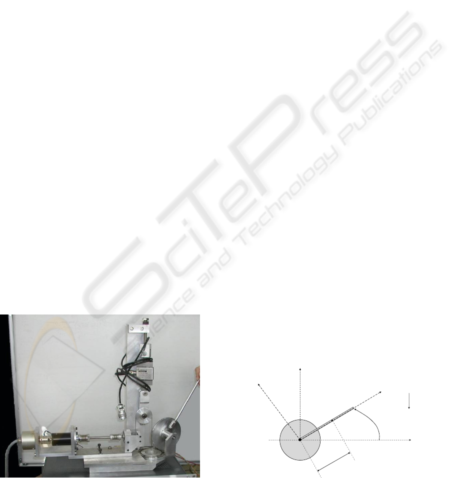
The interface to be identified is presented Figure 1.

It consists of synchronous machine and a handle

actuated thanks to a cable transmission. This type of

transmission is a good comprise between friction,

slippage and losses. The modelling and the

identification are made under the rigid model

assumption. Naturally, the authors have checked that

this hypothesis is valid in the case of this study.

The modelling and the identification of the

synchronous machine are given in (Khatounian et al,

2006).

Figure 1: Presentation of the interface to be identified.

The frames defined to model the interface are

presented Figure 2. The inverse dynamic model is

given by the following equation:

fYX

gsin(q)Mgcos(q)MqJΓ Γ+

−



(16)

where q and



are respectively the joint position and

acceleration, J is the global inertia of the system.

The torque Γ is calculated through the current

measurement. We have verified that we have

Γ=NK

I, where N is the gear ratio, K

the torque

constant and I the measured current. More details

about the implemented control law can be found in

(Khatounian et al, 2006).

The friction torque Γ

was measured according to

the method developed by (Spetch and Isermann,

1988), which consists in measuring the torque at

different constant speeds and eliminating all

transient modes. Figure 3 shows that the friction

model can be considered at non-zero velocity as the

following, where

)qsign(



is the sign function of the

velocity



, and f

, f

denote the Coulomb and

viscous friction coefficients.

)qsign(fqfΓ

cvf



(17)

The dynamic model can be thus written as a

sampled linear form:

Γ = W X (18)

⎥

⎦

⎤

⎢

⎣

⎡

−

)qsign(q)gsin(q)gcos(qq

rrrrr

11111



#####



⎥

⎦

⎤

⎢

⎣

⎡

#Y and

[

]

cvYX

ffMMJ=X .

In this simple case, the parameters J, M

, M

, f

and f

constitute the set of base parameters (QR

decomposition confirms that).

Figure 2: Notations and frames used for modelling the

interface.

ICINCO 2007 - International Conference on Informatics in Control, Automation and Robotics

344

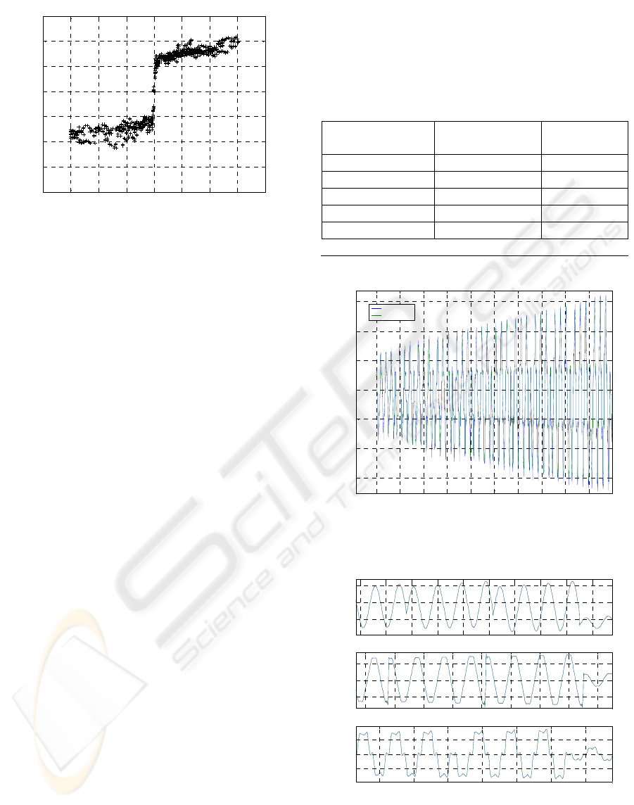
-20 -15 -10 -5 0 5 10 15 20

-0.2

-0.15

-0.1

-0.05

0.05

0.1

0.15

Frictions torque measured

Velocity rads-1

Torque Nm

Figure 3: Friction torque measured.

3.2 Identification of the Base

Parameters

3.2.1 LS Method

Current I and joint position q were measured, with a

sampling period of 240μs. Exciting trajectory

consists of trapezoidal speed reference. This

trajectory was chosen because it is equivalent to a

rectangular trajectory for the joint acceleration. It

allows the estimation of the inertia term due to the

change of the acceleration sign, of the gravitational

and viscous friction terms because the velocity is

constant over a period and of the Coulomb term due

to the change of sign of the velocity. Vectors



and



were derived from the position vector q, and all

data were filtered as described in section 2.2.2.

Because of the friction model, the velocities close to

zero are eliminated.

The cut-off frequency of the butterworth filter and

of the decimate filter is close to 20Hz. This value

can be calculated thanks to a spectral analysis of the

data. In our case one has ω

dyn

close to 2Hz. Thus

with the rule of thumb ω

>10*ω

dyn

, we retrieve the

value given above.

The identified values of the mechanical parameters

are summed up in Table 1.

The conditioning number of W is close to 30.

Hence, the system is well conditioned and the

designed trajectories are enough exciting.

Direct comparisons have been performed. These

tests consist in comparing the measured and the

estimated torques just after the identification

procedure. An example is illustrated Figure 4.

Notice that the estimated torque follows the

measured torque closely.

Finally, we simulate the system by means of a

SIMULINK model. We use the same speed

references and the differential equation given by

(15) is solved with the Euler’s method (ODE 1). The

step time integrator is of 240μs. Figure 5 shows the

measured and the simulated states. They are close to

each others.

Table 1: Estimated mechanical parameter values.

Mechanical

parameters

Estimated

values

Relative

deviation %

J (kg.m²) 1,45.10

-3

0,5

(kg.m) 2,2.10

-3

5,0

(kg.m) 0,9.10

-3

8,7

(Nm.s.rad

-1

)

2,4.10

-3

2,6

(Nm) 5,9.10

-2

0.8

Cond(W) = 30

0 200 400 600 800 1000 1200 1400 1600 1800

-0.3

-0.2

-0.1

0.1

0.2

0.3

Direct Validation

Mes ured

Estimated

Figure 4: Comparison between the measured and

estimated torque calculated through the LS technique.

1550 1600 1650 1700 1750 1800 1850 1900 1950 2000

-1

Measured and Si mulat ed Posi ti on

rad

1600 1650 1700 1750 1800 1850 1900 1950 2000

-10

Measured and Si mulat ed Velocity

rads-1

1700 1750 1800 1850 1900 1950 2000

-100

100

Measured and Simulated Accelerat ion

rads-2

Figure 5: Comparison between the measured states (blue)

and the simulated states (green).

COMPARISON OF TWO IDENTIFICATION TECHNIQUES: THEORY AND APPLICATION

345

It comes that the LS technique identification gives

interesting and reliable results even if the

assumptions on the noise model are violated.

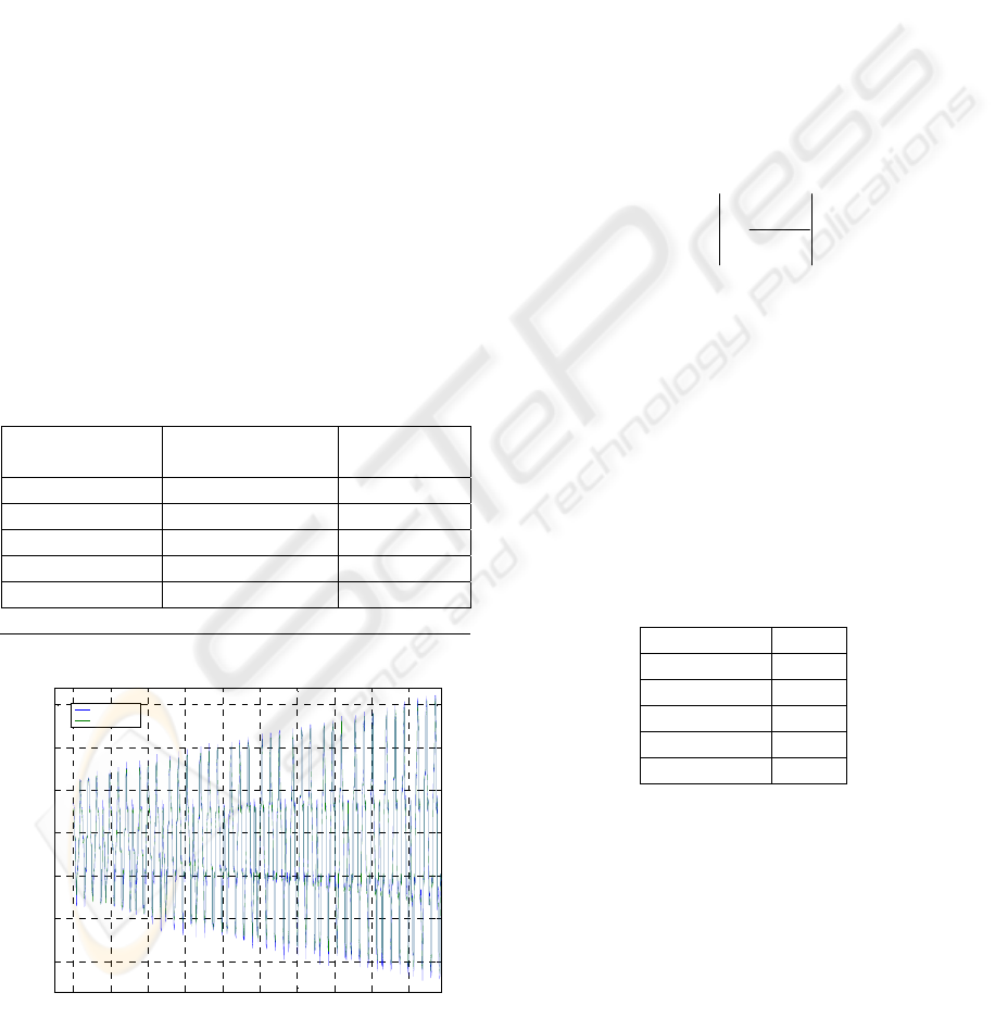
3.2.2 SRIV Method

As explained section 2.3, the instrument matrix is

built with the simulated states (see previous section

for the simulation parameters) and the algorithm is

initialized with the values given in Table 1. The

parameters are estimated thanks to (14). These

values do not vary consequently (only 2 steps are

enough to decrease the correlation between the

instrument matrix and the noise on the system). The

results are summed up in Table 2.

We have also performed direct comparison (Figure

6). Once again, the estimated torque follows the

measured torque closely. As an expected result, the

SRIV method gives reliable and interesting results

and can be used to identify inertial parameters of

robots. The results given Table 2 are close to those

exposed Table 1. That means that, in this case, the

LS method detailed section 2.2 is as efficient as the

SRIV technique detailed section 2.3.

Table 2: Estimated mechanical parameter values

calculated through the SRIV method after 5 steps.

Mechanical

parameters

Estimated values Relative

deviation %

J (kg.m²) 1,45.10

-3

0,4

(kg.m) 2,2.10

-3

5,0

(kg.m) 0,9.10

-3

8,2

(Nm.s.rad

-1

)

1,9.10

-3

3,5

(Nm) 6,3.10

-2

0.8

Cond(W) = 30

0 200 400 600 800 1000 1200 1400 1600 1800

-0.3

-0.2

-0.1

0.1

0.2

0.3

Direct Validation

Mes ured

Estimated

Figure 6: Comparison between the measured and

estimated torque calculated through the SRIV.

4 DISCUSSION

In the case of this study, the experimental results

tend to prove that the identification technique

developed by the IRCCyN robotic team is as

efficient and consistent as the SRIV method. This

mainly due to the data treatment described section

2.2.2. Indeed, it helps the LS estimator: outliers and

leverage points are eliminated while the derivatives

of q are calculated without magnitude and phase

shift. In addition, the data filtering is well designed.

It is interesting to mix both methods. Indeed, with a

simple analysis, we can detect which parameters are

sensitive to noise measurement, noise modelling,

high frequency disturbances…

To do so, we introduce an estimation relative error

given by (19):

LSj

SRIVj

1100%e −=

(19)

Where

SRIVj

is the j

parameter estimated by

means of the SRIV method and

LSj

is the j

parameter estimated thanks to the LS technique. The

results are summed up in Table 3.

In our case, only the parameters of friction torque

are quite sensitive. This is mainly due to the fact that

they “see” all undesirable effects such as torque

ripple, cable wear and imperfect contacts which are

not modelled. Hence, that proves the interest of this

approach and the use of the SRIV method.

Table 3: Estimation relative error.

Parameter %e

J (kg.m²) 0,1 %

Mx (kg.m) 0,2 %

My (kg.m) 1,3 %

fv (Nm.s.rad

-1

) 20 %

fc (Nm) 7,3 %

During the experiments, it is appeared that the

SRIV could be helpful when we are not familiar

with the data filtering. We know that the LS

estimators are sensitive to noises filtering and if the

filtering is not well designed, the results could be

controversial. These results will be published in a

later publication.

ICINCO 2007 - International Conference on Informatics in Control, Automation and Robotics

346

5 CONCLUSION

In this paper, two identification methods have been

tested and compared: the first based on the ordinary

LS technique associated with an appropriate data

treatment and the second based on the SRIV method.

Both methods give interesting and reliable results.

Hence, we can choose these techniques for a

parametric identification.

In addition, the authors have introduced a simple

calculation which enables us to know the parameters

which are sensitive to noises and undesirable effects.

Future works concern the use of both techniques to

identify a 6 degrees of freedom robot.

REFERENCES

Garnier H., Gilson M. and Huselstein E., 2003.

“Developments for the MATLAB CONTSID

toolbox”, In: 13th IFAC Symposium on System

Identification, SYSID 2003, Rotterdam Netherlands,

August 2003, pp. 1007-1012

Garnier H., Gilson M. and Cervellin O., 2006. “Latest

developments for the MATLAB CONTSID toolbox”,

In: 14th IFAC Symposium on System Identification,

SYSID 2006, Newcastle Australia, March 2006, pp.

714-719

Gautier M. and Khalil W., 1990. "Direct calculation of

minimum set of inertial parameters of serial robots",

IEEE Transactions on Robotics and Automation, Vol.

6(3), June 1990

Gautier M. and Khalil W., 1991. “Exciting trajectories for

the identification of base inertial parameters of

robots”, In: Proc. Of the 30

Conf. on Decision and

Control, Brigthon, England, December 1991, pp. 494-

499

Gautier M., 1997. “Dynamic identification of robots with

power model”, Proc. IEEE Int. Conf. on Robotics and

Automation, Albuquerque, 1997, p. 1922-1927

Gautier M., Khalil W. and Restrepo P. P., 1995.

“Identification of the dynamic parameters of a closed

loop robot”, Proc. IEEE on Int. Conf. on Robotics and

Automation, Nagoya, may 1995, p. 3045-3050

Gilson M., Garnier H., Young P.C. and Van den Hof P.,

2006. “A refined IV method for closed loop system

identification”, In: 14th IFAC Symposium on System

Identification, SYSID 2006, Newcastle Australia,

March 2006, pp. 903-908

Hampel F.R., 1971. “A general qualitative definition of

robustness”, Annals of Mathematical Statistics, 42,

1887-1896, 1971

Huber P.J., 1981. “Robust statistics”, Wiley, New-York,

1981

Janot A., Bidard C., Gautier M., Keller D. and Perrot Y.,

2006. “Modélisation, Identification d’une Interface

Médicale”, Journées Identification et Modélisation

Expérimentale 2006, Poitiers, November 2006

Khatounian F., Moreau S., Monmasson E., Janot A. and

Louveau F., 2006. “Simultaneous Identification of the

Inertial Rotor Position and Electrical Parameters of a

PMSM for a Haptic Interface”, In: 12

EPE-PEMC

Conference, Portoroz, Slovenia, August September

2006, CD-ROM, ISBN 1-4244-0121-6

Lemaire Ch.E., Vandanjon P.O., Gautier M. and Lemaire

Ch., 2006. “Dynamic Identification of a Vibratory

Asphalt Compactor for Contact Efforts Estimation”,

In: 14th IFAC Symposium on System Identification,

SYSID 2006, Newcastle Australia, March 2006,pp.

973-978

Mili L., Phaniraj V. and Rousseeuw P.J., 1990. “Robust

estimation theory for bad data diagnostics in electrical

power systems”, In: C. T. Leondes editor, Control and

Dynamic Systems:Advances in Theory and

Applications, pp. 271-325, San Diego 1990, Academic

Press

Mili L., Cheniae M.G., Vichare N.S. and Rousseeuw P.J.,

1996. “Robust state estimation based on projection

statistics”, IEEE Trans. On Power Systems, 11(2),

1118-1127, 1996

Specht R., and Isermann R., 1988. “On-line identification

of inertia, friction and gravitational forces applied to

an industrial robot”, Proc. IFAC Symp. on Robot

Control, SYROCO’88, 1988, p. 88.1-88.6

Young P.C. and Jakeman A.J., 1979. Refined instrumental

variable methods of time-series analysis: Part 1, SISO

systems, International Journal of Control, 29:1-30,

1979

Young P.C., 2006. “An instrumental variable approach to

ARMA model identification and estimation”, In: 14th

IFAC Symposium on System Identification, SYSID

2006, Newcastle Australia, March 2006, pp. 410-415

COMPARISON OF TWO IDENTIFICATION TECHNIQUES: THEORY AND APPLICATION

347