BLIND TWO-THERMOCOUPLE SENSOR

CHARACTERISATION

Peter C. Hung, Seán F. McLoone

Department of Electronic Engineering, National Unviersity of Ireland Maynooth, Maynooth, Co. Kildare, Ireland

George W. Irwin, Robert J. Kee

Virtual Engineering Centre, Queen’s University Belfast, Belfast, Northern Ireland, BT9 5HN

Keywords: Sensor, system identification, thermocouple, blind deconvolution.

Abstract: Thermocouples are one of the most popular devices for temperature measurement in many mechatronic

implementations. However, large wire diameters are required to withstand harsh environments and

consequently the sensor bandwidth is reduced. This paper describes a novel algorithmic compensation

technique based on blind deconvolution to address this loss of high frequency signal components using the

outputs from two thermocouples. In particular, a cross-relation blind deconvolution for parameter

estimation is proposed. A feature of this approach, unlike previous methods, is that no a priori assumption

is made about the time constant ratio of the two thermocouples. The advantages, including small estimation

variance, are highlighted using results from simulation studies.

1 INTRODUCTION

There is a growing trend towards the integration of

different types of sensors and actuators with

information processing (Isermann, 2005).

Commercial and industrial applications increasingly

demand dynamic temperature measurement when

advanced mechatronic components are incorporated.

In the automotive industry for example, accurate and

reliable measurement of exhaust gas temperature is

required for the regeneration of diesel particulate

filters (DPF), and for the evaluation of the

combustion performance of internal combustion

engines (Kee and Blair, 1994).

Fast response temperature measurement can be

performed using techniques such as Coherent Anti-

Stokes Spectroscopy, Laser-Induced Fluorescence

and Infrared Pyrometry. However, these are

expensive, difficult to calibrate and maintain and are

therefore impractical for wide-scale deployment

outside the laboratory (Hung et al., 2005a).

Thermocouples are widely used for temperature

measurement due to their high permissible working

limit and good linear temperature dependence. In

addition, their low cost, robustness, ease of

installation and reliability means that there are many

situations in which thermocouples are indeed the

only suitable choice. Unfortunately, their design

involves a compromise between robustness and

speed of response which poses major problems when

measuring temperature fluctuations with high

frequency signal components.

To remove the effect of the sensor on the

measured quantity in such conditions, compensation

of the thermocouple measurement is desirable.

Usually, this compensation involves two stages:

thermocouple characterisation followed by

temperature reconstruction. Reconstruction is a

process of restoring the unknown fluid temperature

from thermocouple outputs using either software

techniques or hardware. This paper will concentrate

on the first stage, since effective and reliable

characterisation is essential for achieving

satisfactory temperature reconstruction.

In an attempt to improve existing

characterisation of thermocouples, this paper

proposes a novel technique based on the cross-

relation method (Liu et al., 1993) from the field of

blind deconvolution put forward by Sato (1975).

Compared to other algorithms, simulations suggest

C. Hung P., F. McLoone S., W. Irwin G. and J. Kee R. (2007).

BLIND TWO-THERMOCOUPLE SENSOR CHARACTERISATION.

In Proceedings of the Fourth International Conference on Informatics in Control, Automation and Robotics, pages 10-16

DOI: 10.5220/0001627200100016

 SciTePress

that the proposed method gives estimations with

lower variance even in environments with moderate

amount of noise.

This paper is organised as follows: Section 2

introduces the background of two-thermocouple

characterisation. Section 3 proposes the cross-

relation method and shows how it can be applied to

this problem. Simulation results are presented in

Section 4 while conclusions follow in Section 5.

2 DIFFERENCE EQUATION

SENSOR

CHARACTERISATION

2.1 Thermocouple Modelling

Assuming some criteria regarding to the

construction of thermocouples are satisfied (Forney

and Fralick, 1994; Tagawa and Ohta, 1997), a first-

order lag model with time constant

and unity gain

can represent the frequency response of a fine-wire

thermocouple (Petit, 1982). This simplified model

can be written mathematically as

)()()(

fluid

tTtTtT



(1)

Here the original fluid temperature

fluid

T can be

reconstructed if

, the thermocouple output )(tT

and its derivative are available. In practice, this

direct approach is infeasible as

)(tT contains noise

and its derivative is difficult to estimate accurately.

More importantly, it is generally not possible to

obtain a reliable a priori estimate of

, related to

their thermocouple bandwidth

(2)

which, in turn, is a function of thermocouple wire

diameter

and fluid velocity

∝

. (3)

Hence,

varies as a function of operating

conditions. Clearly, a single-thermocouple does not

provide sufficient information for in situ estimation.

Equation (3) highlights the fundamental trade-off

that exists when using thermocouples. Large wire

diameters are usually employed to withstand harsh

environments such as engine combustion systems,

but these results in thermocouples with low

bandwidth, typically

< 1 Hz. In these situations

high frequency temperature transients are lost with

the thermocouple output significantly attenuated and

phase-shifted compared to

fluid

T Consequently,

appropriate compensation of the thermocouple

measurement is needed to restore the high frequency

fluctuations.

2.2 Two-Thermocouple Sensor

Characterisation

In 1936 Pfriem suggested using two thermocouples

with different time constants to obtain in situ sensor

characterisation. Since then, various thermocouple

compensation techniques incorporating this idea

have been proposed in an attempt to achieve

accurate and robust fluid temperature compensation

(Forney and Fralick, 1994; Tagawa and Ohta, 1997;

Kee et al., 1999; Hung et al., 2003, 2005a, 2005b).

However, the performance of all these algorithms

deteriorates rapidly with increasing noise power, and

many are susceptible to singularities and sensitive to

offsets (Kee et al., 2006). It would be very useful

from the implementation point of view to know

when the characterisations are not reliable.

Some of these two-thermocouple methods rely

on the restrictive assumption that the ratio of the

thermocouple time constants

1( <

definition) is known a priori. Hung et al. (2003,

2005a, 2005b) develop difference equation methods

that do not require any a priori assumption about the

time constant ratio.

The equivalent discrete time representation for

the thermocouple model (2) is:

)1()1()(

fluid

−

kbTkaTkT ,

(4)

where

and

are difference equation ARX

parameters and

k is the sample instant. The discrete

time equivalent of

is defined as

bb .

(5)

Here subscripts 1 and 2 are used to distinguish

between signals from different thermocouples.

Assuming ZOHs and a sampling interval

, the

parameters of the discrete and continuous time

thermocouple models are related by

BLIND TWO-THERMOCOUPLE SENSOR CHARACTERISATION

aba

−=−= 1,)exp(

(6)

Since two sets of (4) are available from each

thermocouple outputs

)(

kT and ),(

kT a beta

model (Hung,

et al., 2005) can be formulated by

eliminating

fluid

T from (4) to become

12212

−

Δ+Δ=Δ

kkk

TbTT

(7)

where the pseudo-sensor output

Δ and inputs

Δ and

−

T are defined as

).1()1(

)1()(

222

111

−−−=Δ

−−=Δ

−

kTkTT

(8)

For an

M-sample data set (7) can be expressed in

ARX vector form

XθY =

(9)

with

.][and],[,

1212

Tkkk

=ΔΔ=Δ=

−

θTTXTY

Here

TΔ ,

TΔ and

−

T are vectors containing

M-1 samples of the corresponding composite signals

Δ ,

Δ and

−

T .

Due to the form of the composite input and

output signals, the noise terms in the

X and Y data

blocks are no longer independent. The result is that

conventional least-squares and total least-squares

both generate biased parameter estimates even when

the measurement noise on the thermocouples is

independent. It has been shown that generalised total

least-squares (GTLS) on the other hand, can produce

unbiased parameter estimate

that outperforms

other difference equation based methods. One of the

reasons can be traced back to the use of

, which

enhanced the model stability during parameter

estimation (McLoone

et al., 2006).

Unfortunately, the

GTLS−

approach

occasionally returns unreasonable

estimates as

will be illustrated in Section 4. This is caused by the

sensitivity of GTLS to violations in the underlying

theoretical assumptions with composite signals

(Huffel and Vandewalle, 1991), plus ill-conditioning

of the noise correlation matrix. The blind

deconvolution approach is considered here to isolate

these invalid

3 BLIND SENSOR

CHARACTERISATION

One of the best known deterministic blind

deconvolution approaches is the method of cross-

relation (CR) proposed by Liu

et al. (1993). Such

techniques exploit the information provided by

output measurements from multiple systems of

known structure but unknown parameters, for the

same input signal.

This new approach to characterisation of

thermocouples is completely different from those in

Section 2. As commutation is a fundamental

assumption for the method of cross-relation, the

thermocouple models are both assumed to be linear.

This is reasonably realistic as long as the

thermocouples concerned are used within well-

defined temperature ranges. Nonetheless,

linearisation can easily be carried out using either

the data capture hardware or software, even if the

thermocouple response is nonlinear. Further, the

approach requires constant model parameters,

therefore the fluid flow velocity

is assumed to be

constant, such that the two thermocouple time

constants

and

are time-invariant.

Figure 1: Two-thermocouple cross-relation characterisation.

)(

unknown system

)(

fluid

)(

ICINCO 2007 - International Conference on Informatics in Control, Automation and Robotics

3.1 Two-Thermocouple Sensor

Characterisation

By exploiting the commutative relationship between

linear systems, a novel two-themocouple

characterisation scheme is proposed as follows.

Since the fluid temperature

fluid

T is unknown, the

two thermocouple output signals

T and

T are

passed through two different synthetic

thermocouples as shown in Fig. 1. These are also

modelled by (1) and can be expressed in first-order

transfer function as:

)(

ττ

(10)

where

is the estimate of the thermocouple

transfer function

The unknown thermocouple

time constant parameters can then be estimated as

and

using the cross-relation method,

illustrated in Fig. 1. Here the cross-relation error

signal,

)()(

2112

tTtTe −= is used to define a mean-

square-error cost function

,})]()({[

}{)

(

2112

212

ττ

∀−=

tTtTE

eEJ

(11)

Equation (11) is then minimised with respect to

and

to yield the estimates of the unknown

thermocouple time constants. Clearly, the cross-

relation cost function

)

(

212

J is zero when

= and .

= In practice it will not be

possible to obtain an exact match between

T and

T due to measurement noise and other factors such

as thermocouple modelling inaccuracy and

violations of the assumption that the two

thermocouples are experiencing identical

environmental conditions.

Xiu

et al. (1995) suggest that one of the

necessary conditions for multiple finite-impulse-

response channels to be identifiable is that their

transfer function polynomial do not share common

roots. Applying this condition to the two-

thermocouple characterisation problem corresponds

to requiring that the time constants, and hence the

diameters (3), of the thermocouples are different,

that is

2121

dd ≠⇒≠

(12)

Not surprsingly, this requirement is consistent with

all other two-thermocouple characterisation

techniques mentioned in Section 2. Thus, cross-

relation deconvolution converts the problem of

sensor characterisation into an optimisation one.

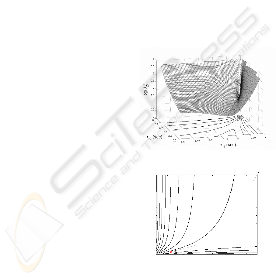
3.2 Cost Function

A 3-D surface plot and a contour map of a typical

)

(

212

J cost function are shown in Figs. 2 and 3.

Unfortunately,

)

(

212

J is not quadratic and

cannot therefore be minimised using linear least-

squares. Fig. 3 shows that the cross-relation cost

function is highly non-quadratic away from the

minimum corresponding to the value of the true time

constants.

Figure 2: Three-dimensional plot of log(J

0.05 0.1 0.15 0.2 0.25 0.3 0.35 0.4 0.45 0.5

0.05

0.1

0.15

0.2

0.25

0.3

0.35

0.4

0.45

0.5

(sec)

local

minimum

global

minimum

at infinity

Figure 3: Contour plot of J

(cross: local minimum).

More importantly, the cost function has a second

minimum when both time constant values approach

infinity. Under these conditions, both low-pass

filters (10) take infinite amounts of time to respond.

BLIND TWO-THERMOCOUPLE SENSOR CHARACTERISATION

In other words, they are effectively open-circuited

and their differences will always be zero. The

existence of this minimum applies regardless of the

noise conditions or any violations of the modelling

assumptions. The minimum at infinity is thus in fact

the global minimum, while the true time constant

value is located at a local minimum. In the absence

of noise,

=J at both the global and local minima.

In addition, the narrow basin of attraction of the

desired local minimum coupled with the global

minimum at infinity has serious implications for

optimisation complexity since search bounds have to

be carefully selected to avoid divergence of gradient

search algorithms to the global minimum.

Consequently, in this study a robust, but inefficient,

grid based search has been adopted to avoid these

issues. To reduce the associated computational load

different step sizes are used for each time constant.

Noting from Fig. 3 that, at least locally,

ττ

∂

(13)

it can be concluded that the cost function is more

sensitive to changes in the smaller thermocouple

time constant; hence greater accuracy is required in

estimating this value.

4 SIMULATION RESULTS

A MATLAB® simulation of a two-thermocouple

probe system (Fig. 4) was used to evaluate the

performance of the proposed cross-relation (CR)

blind sensor characterisation. Thermocouples 1 and

2 were modelled as first-order low-pass filters

according to (1) with time constants

8.23

and

8.116

ms respectively. The simulated fluid

temperature was varied sinusoidally according to

5.50)20sin(5.16)(

fluid

+= ttT

(14)

and the resulting temperature measurements sampled

every 2 ms. Each simulation ran for 5 s.

The level of zero-mean white Gaussian

measurement noise added to the thermocouple

signals is described by the noise level

L , defined as

,2,1,%100

)var(

fluid

=⋅= i

(15)

Figure 4: Simulated two-thermocouple measurement

system.

where

n and

n are the noises added to the

thermocouples. For a given

L , the algorithm

performance was assessed in terms of percentage

estimation errors:

%100

⋅

−

e .

(16)

To reduce the time required for completing the

simulation, the following search ranges and intervals

(13) were chosen for the cross-relation (CR)

algorithm:

ms. 2.5every at ms;130

100

ms, 0.5every at ms;30

(17)

Of particular importance was the removal of the

first 1000 data samples before computing

)

(

212

J , using the remaining 1500 sets of CR

outputs

and

T . This was required to eliminate

the effect of transients on parameter estimation

accuracy during each iteration of CR simulation

(Fig. 1). The number of samples removed was

estimated to exceed the 98% settling time for the

system (i.e. five times the largest time constant

)

which equated to about 0.6 s or 300 samples.

The resulting means and standard deviations of

the parameter estimation error (16), for both

GTLS

−

(Section 2.2) and CR (Section 3.1)

algorithms are shown in Fig. 5. Note results for

are similar to those illustrated for

and are thus

omitted.

)(

fluid

ICINCO 2007 - International Conference on Informatics in Control, Automation and Robotics

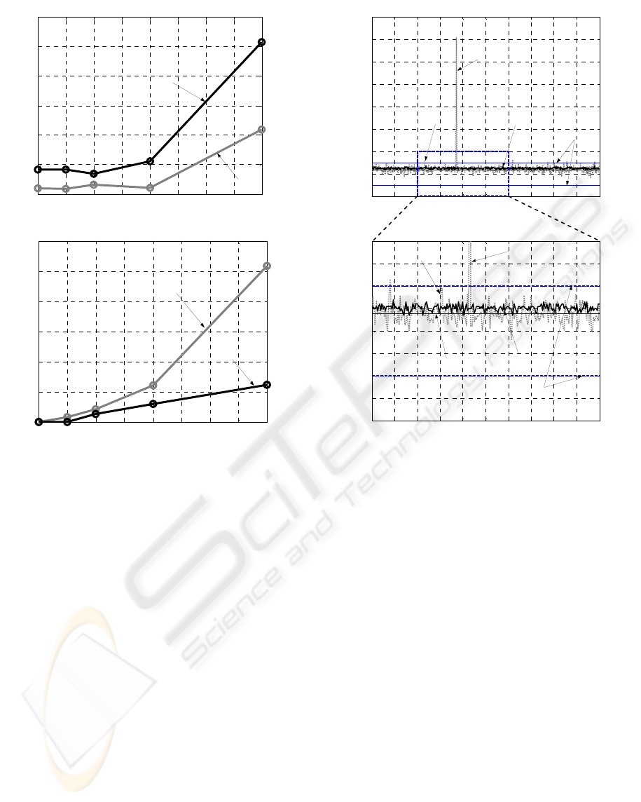
Figure 5: (a) Means and (b) standard deviations of e of

averaged over 100 Monte-Carlo runs.

These results suggset that CR produces biased

parameter estimates since their expected mean errors

are greater than that of

GTLS−

. However, the

estimation standard deviations of CR are less than

that of

GTLS−

With regard to the search intervals taken for CR,

two issues need to be considered when looking at the

graphs. Firstly, a major contribution to the CR bias

comes from the low resolution of the search grid

used. Since, when

8.23

ms, an interval of 0.5

ms represents an ‘artificial’ estimation bias of up to

2.1%. This can be reduced if a finer search grid is

employed, at the expense of increasing the already

heavy computation load. Similarly, the CR standard

deviation errors may be 2.1% larger than the

reported values because of the finite resolution

employed, although this is unlikely due to the

intrinsic noise-filtering capability of CR.

The noise-resilient property of CR compared to

GTLS is further highlighted in Fig. 6, where 500

Monte-Carlo simulations were performed. It can be

seen that one unreasonable

value was returned by

GTLS

−

while the CR approach is well-behaved,

although its estimate is asymptotically biased.

Hence, CR can be used to verify whether a GTLS

estimate is genuine or corrupted by signal outliers,

improving the overall reliability of sensor

characterisation.

5 CONCLUSIONS

A novel cross-relation (CR) sensor characterisation

method has been presented. It does not require a

priori knowledge of the thermocouple time constant

ratio

, as required in many other characterisation

algorithms. CR is more noise-tolerant in the sense of

reduced parameter estimation variance when

compared to the alternatives such as

GTLS−

. The

robustness arises because the CR process involves

passing each thermocouple output through a first-

order block, which removes, at least partially,

Figure 6: 500 Monte-Carlo runs of

of GTLS−

and

CR, where (b) is a magnified version of (a).

0 50 100 150 200 250 300 350 400 450 500

0.02

0.04

0.06

0.08

0.1

0.12

0.14

0.16

Monte-Carlo iteration

estimated

(sec)

-GTLS

unreasonable

-GTLS estimate

CR search

range

(a)

100 120 140 160 180 200 220 240 260 280 300

0.005

0.01

0.015

0.02

0.025

0.03

0.035

0.04

Monte-Carlo iteration

estimated

(sec)

-GTLS

unreasonable

-GTLS estimate

CR search

range

(b)

true

= 0.0238 s

0 0.5 1 1.5 2 2.5 3 3.5 4

average error in

(%)

-GTLS

(a)

0 0.5 1 1.5 2 2.5 3 3.5 4

SD error in

(%)

-GTLS

(b)

BLIND TWO-THERMOCOUPLE SENSOR CHARACTERISATION

measurement noise during identification. As a result,

CR can be employed to verify estimation validity,

thereby increasing the overall reliability of other

characterisation methods.

The computational complexity of CR, due to the

inefficient grid based search used in this study,

means that it is most appropriate for offline sensor

characterisation. Further investigations include ways

to speed up the computation and reduce the

estimation bias.

ACKNOWLEDGEMENTS

The authors wish to acknowledge the financial

support of the Virtual Engineering Centre, Queen’s

University Belfast, http://www.vec.qub.ac.uk.

REFERENCES

Forney, L. J., Fralick G. C., 1994. Two wire

thermocouple: Frequency response in constant flow.

Rev. Sci. Instrum., 65, pp 3252-3257.

Hung, P., McLoone, S., Irwin G., Kee, R., 2003. A Total

Least Squares Approach to Sensor Characterisations.

Proc. 13th IFAC Symposium on Sys. Id., Rotterdam,

The Netherlands, pp 337-342.

Hung, P. C., McLoone, S., Irwin G., Kee, R., 2005a. A

difference equation approach to two-thermocouple

sensor characterisation in constant velocity flow

environments. Rev. Sci. Instrum., 76, Paper No.

024902.

Hung, P. C., McLoone, S., Irwin G., Kee, R., 2005b.

Unbiased thermocouple sensor characterisation in

variable flow environments. Proc. 16th IFAC World

Congress, Prague, Czech Republic.

Isermann, R., 2005. Mechatronic Systems – Innovative

Products with Embedded Control. Proc. 16th IFAC

World Congress, Prague, Czech Republic.

Kee, R. J., Blair, G. P., 1994. Acceleration test method for

a high performance two-stroke racing engine. Proc.

SAE Motorsports Conference, Detroit, MI, Paper No.

942478.

Kee, R. J, O'Reilly, P. G., Fleck, R., McEntee, P. T., 1999.

Measurement of Exhaust Gas Temperature in a High

Performance Two-Stroke Engine. SAE Trans. J.

Engines, 107, Paper No. 983072.

Kee, J. K., Hung, P., Fleck, B., Irwin, G., Kenny, R.,

Gaynor, J., McLoone, S., 2006. Fast response exhaust

gas temperature measurement in IC Engines. SAE

2006 World Congress, Detroit, MI, Paper No. 2006-

01-1319.

Liu, H., Xu, G., Tong, L., 1993. A deterministic approach

to blind identification of multichannel FIR systems.

Proc. 27th Asilomar Conference on Signals, Systems

and Computers, Asilomar, CA, pp. 581-584.

McLoone, S., Hung, P., Irwin, G., Kee, R., 2006.

Exploiting A Priori Time Constant Ratio Information

in Difference Equation Two-Thermocouple Sensor

Characterisation. IEEE Sensors J., 6, pp. 1627-1637.

Pfriem, H., 1936. Zue messung verandelisher

temperaturen von ogasen und flussigkeiten. Forsch.

Geb. Ingenieurwes, 7, pp. 85-92.

Petit, C., Gajan, P., Lecordier, J. C., Paranthoen, P., 1982.

Frequency response of fine wire thermocouple. J.

Physics Part E, 15, pp. 760-764.

Sato, Y., 1975. A method of self-recovering equalization

for multilevel amplitude modulation systems. IEEE

Trans. in Communications, 23, pp. 679-682.

Tagawa, M., Ohta, Y., 1997. Two-Thermocouple Probe

for Fluctuating Temperature Measurement in

Combustion – Rational Estimation of Mean and

Fluctuating Time Constants. Combustion and Flame,

109, pp 549-560.

Xu, G., Liu, H., Tong, L., Kailath, T., 1995. A least-

squares approach to blind channel identification. IEEE

Trans. on Signal Processing, 43, pp. 2982-2993.

Van Huffel S., Vandewalle, J., 1991. The Total Least

Squares Problem: Computational Aspects and

Analysis, SIAM, Philadelphia, 1

edition.

ICINCO 2007 - International Conference on Informatics in Control, Automation and Robotics