ON GENERATING GROUND-TRUTH TIME-LAPSE IMAGE

SEQUENCES AND FLOW FIELDS

Vladim

ır Ulman and Jan Huben

Centre for Biomedical Image Analysis, Masaryk University, Botanick

a 68a, Brno 602 00, Czech Republic

Keywords:

Optical ﬂow evaluation, ground-truth ﬂow ﬁeld.

Abstract:

The availability of time-lapse image sequencies accompanied with appropriate ground-truth ﬂow ﬁelds is cru-

cial for quantitative evaluation of any optical ﬂow computation method. Moreover, since these methods are

often part of automatic object-tracking or motion-detection solutions used mainly in robotics and computer vi-

sion, an artiﬁcially generated high-ﬁdelity test data is obviously needed. In this paper, we present a framework

that allows for automatic generation of such image sequences based on real-world model image together with

an artiﬁcial ﬂow ﬁeld. The framework beneﬁts of a two-layered approach in which user-selected foreground

is locally moved and inserted into an artiﬁcially generated background. The background is visually similar to

the input real image while the foreground is extracted from it and so its ﬁdelity is guaranteed. The framework

is capable of generating 2D and 3D image sequences of arbitrary length. A brief discussion as well as an

example of application in optical microscopy imaging is presented.

1 INTRODUCTION

The growing importance of image processing meth-

ods is unquestionable in the ﬁeld of automation and

robotics. Especially, optical ﬂow computation meth-

ods are often involved in solutions adopted in, for in-

stance, autonomous systems and agents, vehicle con-

trol applications, surveillance or live-cell microscopy.

The outcome of these methods is often not the ﬁ-

nal product. It is usually further analyzed by object-

tracking or motion-detection methods (C

edras and

Shah, 1995; Gerlich et al., 2003; Eils and Athale,

2003).

Important is also thorough testing of a particular

method before its application. This is even more evi-

dent due to the continuous development of image ac-

quisition devices, since the usability of given image

processing method is changing with the nature of ex-

amined image data. Veriﬁcation is, therefore, an ob-

vious need.

For the purpose of fully automatic testing one has

to have a large data set together with correct results

prepared. Or, the dataset should be generated online

reasonably fast. A dataset consisting of real images

is obviously the ideal choice. Unfortunately, the real

images do not explicitly provide the ground-truth in-

formation about the motion expressed in the data.

There exist methods that extract such motion in-

formation, for example other, than currently tested,

optical ﬂow methods (Horn and Schunck, 1981; Bar-

ron et al., 1994) or image registration techniques (Zi-

tov

a and Flusser, 2003). Unfortunately, these practi-

cally always incur some sort of error or imprecision in

the ﬂow ﬁeld. The same holds for manually processed

data (Webb et al., 2003), not mentioning the tedious

extraction of ground-truth motion information.

We decided to automatically generate vast amount

of artiﬁcial test images with the stress on their near-

perfect visual similarity to the real data of the ap-

plication in mind. The aim was to conﬁdently test

the reliability of the given optical ﬂow computation

method using this data. Moreover, we wanted to gen-

erate image sequences together with associated ﬂow

ﬁelds reasonably fast (i.e. faster than the execution

of an optical ﬂow computation method) to be able to

simulate the behaviour of real-time decision system

incorporating optical ﬂow computation. Tracking of

a live cell in microscopy can be taken as an exam-

234

Ulman V. and Hubený J. (2007).

ON GENERATING GROUND-TRUTH TIME-LAPSE IMAGE SEQUENCES AND FLOW FIELDS.

In Proceedings of the Fourth International Conference on Informatics in Control, Automation and Robotics, pages 234-239

DOI: 10.5220/0001630202340239

 SciTePress

ple of such a decision-making system. Due to tech-

nology limits the cell can be acquired with only re-

stricted (small) surroundings and needs on-line 2D or

3D tracking (moving the stage with the cell based on

its motion).

The next section gives a motivation to the adopted

solution by means of brief overview of possible ap-

proaches. The third section describes the proposed

framework which automatically generates 2D and 3D

image sequences of arbitrary length. It is followed by

the section in which behaviour and sample image data

for the case of optical microscopy is presented. A 3D

image is considered as a stack of 2D images in this

paper.

2 MOTIVATION

Basically, there are just two possible approaches to

obtain image sequences with ground-truth ﬂow ﬁelds.

One may inspect the real data and manually determine

the ﬂow ﬁeld. Despite the bias (Webb et al., 2003) and

possible errors, this usually leads to a tedious work,

especially, when inspecting 3D image sequences from

a microscope. The other way is to generate sequences

of artiﬁcial images from scratch by exploiting some

prior knowledge of a generated scene. This is usually

accomplished by taking 2D snapshots of a changing

3D scene (Galvin et al., 1998; Barron et al., 1994;

Beauchemin and Barron, 1995). The prior knowledge

is encoded in models which control everything from

the shape of objects, movements, generation of tex-

tures, noise simulation, etc. (Lehmussola et al., 2005;

Young, 1996). This may involve a determination of

many parameters as well as proper understanding of

the modeled system. Once the two consecutive im-

ages are created, the information about movement be-

tween these two can be extracted from the underlying

model and represented in a ﬂow ﬁeld.

We have adopted the approach in which we rather

modify an existing real sample image in order to gen-

erate an image sequence. This enabled us to avoid

most of the modeling process as we shall see later.

Moreover, we could easily create a ﬂow ﬁeld we

were interested in. Consecutive images from the sam-

ple image could be then transformed by using either

backward or forward transformations (Lin and Bar-

ron, 1994). Both transformations are possible. Never-

theless, we observed that forward transformation was

substantially slower. Hence, we described the frame-

work based only on backward transformation in this

paper.

The backward transformation moves the content

of an image with respect to the input ﬂow ﬁeld. The

ﬂow ﬁeld assigns a vector to each voxel in the im-

age. When generating a sequence, the voxel value

is expected to move along its vector into the follow-

ing image. The backward transformation works in the

opposite direction: the preceding image is always cre-

ated. Basically, the voxel at vector’s origin is fetched

into an output image from vector’s end in the input

image. An interpolation in voxel values often occurs

due to real numbers in vectors.

A few drawbacks of the backward transformation

must be taken into account when used. Owing to the

interpolation the transformed image is blurred. The

severity depends on the input ﬂow ﬁeld as well as in-

terpolation method used. Moreover, the blur becomes

more apparent after a few iterative transformations of

the same image. Thus, the number of transformations

should be as low as possible. Another issue appears

when the ﬂow ﬁeld is not continuous. In this case, two

(or even more) vectors may end up in the same posi-

tion which copies the same voxel into distinct places

in the output image. Unfortunately, non-continuous

ﬂow ﬁeld is the case when local movements are to be

simulated. Both drawbacks are demonstrated in the

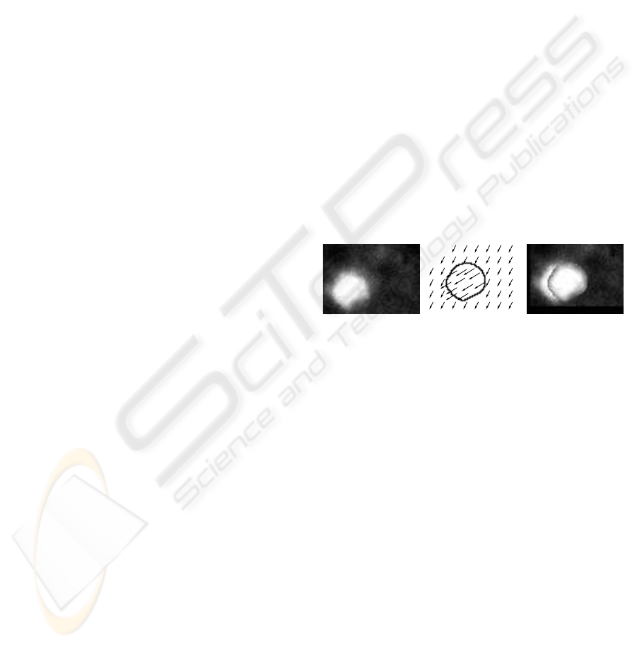
example in Fig. 1.

CA B

Figure 1: Backward transformation. A) An input image. B)

Visualization of the input ﬂow ﬁeld with two homogeneous

regions. C) A transformed image. Notice the blurred corona

as well as the partial copy of the moved object. Images were

enhanced to be seen better.

3 THE FRAMEWORK

In this section we described the framework based

on two-layered component-by-component backward

transformation. The input to the framework was an

real-world sample image, a background mask, a fore-

ground mask and a movements mask. The back-

ground mask denoted what, as a whole, should be

moved in the sample image. The foreground mask de-

noted independent regions (components) in the sam-

ple image that were subjects to local movements.

The movements of components had to remain inside

the movements mask. The output of the framework

was a sequence of artiﬁcially generated images to-

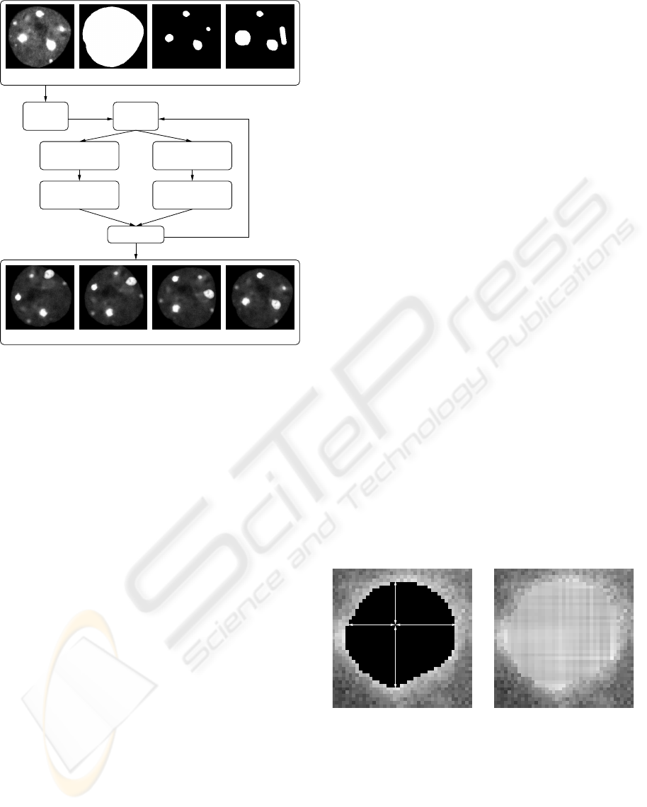
gether with appropriate ﬂow ﬁelds. The schema of the

framework is displayed in Fig. 2. The foreground and

background masks were results of advanced segmen-

tation method (Huben

y and Matula, 2006) which was

ON GENERATING GROUND-TRUTH TIME-LAPSE IMAGE SEQUENCES AND FLOW FIELDS

235

iTH FRAME

BACKGROUND

GENERATION

LOCAL

MOTIONS

FOREGROUND

PREPARATION

INPUT

RANDOM

POOL

GLOBAL

MOTION

BACKGROUND

PREPARATION

OUTPUT

Figure 2: The schema of the framework. From left to right

in INPUT: sample image, background mask, foreground

mask, movements mask; in OUTPUT: examples of 1st,

10th, 20th and 30th image of a generated sequence, respec-

tively. Images were enhanced to be seen better.

initiated with manually thresholded mask images.

The framework was aimed against two obstacles.

Firstly, when foreground component was moved away

from its place, the empty region had to be ﬁlled

in. Therefore, only image regions corresponding to

foreground components could be directly used. The

whole background had to be artiﬁcially generated.

Secondly, several transformations of the same image

data was not acceptable. In order to generate long se-

quences without increasing blur in generated images,

we developed a concept of generating ith image di-

rectly from the sample image instead of the i + 1th

image. Last but not least, owing to the backward

transformation property the framework generated im-

age sequence from the last to the ﬁrst image.

The random pool was the initiating step of the pro-

cess. Here, speciﬁc voxels from the sample image

were collected and stored into a separate image. Vox-

els had to lay inside the background mask and out-

side the foreground mask. The mean intensity value

µ over these voxels was computed. The selection was

then even restricted. In the separate image, the pool,

remained only such voxel which intensity value was

inside the interval (µ− σ, µ+kσ) where σ and k were

supplied manually. We set σ = 11 and k = 3/2 to ﬁt

the real histogram better. This will probably change

when different sort of images is generated.

A simulation of some global movement of the en-

tire sample image was achieved in the unit global mo-

tion. In this unit, the ﬂow ﬁeld for the ith frame was

formed for the ﬁrst time. The foreground and back-

ground masks as well as movements mask were trans-

formed according to this ﬂow ﬁeld. There was a zero

ﬂow ﬁeld created when processing the last image of

the sequence, i.e. the ﬁrst image created by the frame-

work.

The generation of background started from prepa-

ration of the sample image. The sample image had to

be positioned to ﬁt the background mask. We made

use of a special ﬂow ﬁeld for that purpose. This ﬂow

ﬁeld was concatenated to the ﬂow created in the pre-

vious unit and the result was kept until the next se-

quence image is considered. Copy of sample image

was transformed according to this special ﬂow ﬁeld.

Note that the backward transformation may be used

for concatenation of ﬂow ﬁelds if we store ﬂow vec-

tor’s elements in separate images. The concatenated

ﬂow is transformed and added to the ﬂow.

A new similar background was created in two

steps. The foreground components were removed

from the transformed copy of sample image and the

holes were ﬁlled in as described in Fig. 3. The result

was ﬁltered in order to estimate local averages. We

used the 9× 9 ﬁlter of ones which still reﬂected local

intensity values sensitively, yet the ﬁltered image was

smooth. In the second step, the background mask was

ﬁlled in with randomly chosen values from the pool

created in the random pool unit. Finally, correspond-

ing local average subtracted to the value of the mean µ

was added to each voxel within the background mask.

This ensured the high ﬁdelity of the generated texture.

Figure 3: The ﬁlling of removed foreground regions. A)

For each examined voxel, nearest voxel in each direction

outside the black region is found and the distance is deter-

mined. A weighted average of 1/distance-based values is

supplied. B) The result of such ﬁlling.

The foreground mask was ﬁrst decomposed into

independent components in the local motions unit.

Each one is treated separately. A translating motion

vector was randomly chosen from all such vectors that

keep the component within the movement mask. We

ICINCO 2007 - International Conference on Informatics in Control, Automation and Robotics

236

also made use of user supplied parameter for maxi-

mum allowed length of motion vector which enabled

us to control the magnitude of independent local mo-

tions. A temporary ﬂow ﬁeld was created and uni-

formly ﬁlled with this vector. The mask of this com-

ponent only and a copy of the ith ﬂow ﬁeld were trans-

formed according to this uniform ﬂow. This moved

the component mask and prepared the concatenation

of the corresponding region of the ﬂow ﬁeld. The

concatenation was ﬁnished by pasting this region fol-

lowed by addition of chosen ﬂow vector to each vec-

tor inside the region into the ith ﬂow. Note that more

complex foreground movement may be used by sub-

stituting any smooth ﬂow ﬁeld for the uniform one

as well as corresponding vectors should be added in-

stead of constantly adding the chosen one. After all,

new foreground mask was created by merging all sin-

gle locally moved masks.

In the foreground preparation unit, similarly to

the background preparation, another special ﬂow ﬁeld

was used. It was again concatenated to the current

ith ﬂow and the result was stored for the next frame-

work’s iteration. Another copy of sample image was

transformed according to this another special ﬂow

ﬁeld to position the foreground texture.

In the ith frame unit, the foreground regions were

extracted from the transformed copy of sample im-

ages. The extraction was driven by the new fore-

ground mask which was dilated (extended) only for

that purpose beforehand. Finally, the ith image was

ﬁnished by weighted insertion (for details refer to (Ul-

man, 2005)) of the extracted foreground into the artiﬁ-

cially generated background. The weights were com-

puted by thresholding the distance transformed (we

used (Saito and Toriwaki, 1994)) foreground mask.

An illustration of the whole process is shown in Fig. 4.

4 RESULTS

We implemented and tested the presented frame-

work in C++ and in two versions. The ﬁrst version

created only image pairs while the second version cre-

ated arbitrarily long image sequences. It was imple-

mented with both backward and forward transforma-

tions. We observed that for 2D images the forward

variant was up to two orders of magnitude slower than

the backward variant. Therefore, the second version

was implemented based only on backward transfor-

mation. The program required less then 5 minutes on

Pentium4 2.6GHz for computation of a sequence of

50 images with 10 independent foreground regions.

The generator was tested on several different 2D

real-world images and one real-world 3D image. All

generated images were inspected. The framework

generates every last image in the sequence as a re-

placement for the sample image. Thus, we com-

puted correlation coefﬁcient (Corr.), average abso-

lute difference (Avg. diff.) and root mean squared

(RMS) differences. The results are summarized in

Table 1. The generator achieved minimal value of

0.98 for correlation. This quantitatively supports our

observations that generated images are very close to

their originals. The suggested framework also guaran-

tees exactly one transformation of the sample image,

hence the quality of the foreground texture is best pos-

sible thorough the sequence. Refer to Fig. 5 for ex-

ample of 3 images of a 50 images long sequence. A

decent improvement was also observed when an arti-

ﬁcial background of 3D image was formed in a slice-

by-slice manner, see rows C and D in Table 1. In the

case of row D, a separate random pools and mean val-

ues were used for each slice of the 3D image.

Inappropriately created foreground mask may em-

phasize the borders of extracted foreground when

inserted into artiﬁcial background. The weighted

foreground insertion was observed to give visually

better results. Table 1 quantitatively supports our

claim: merging the foreground components accord-

ing to twice dilated foreground mask was comparable

to the plain overlaying of foreground components ac-

cording to non-modiﬁed masks.

The use of user-supplied movements mask pre-

vented the foreground components from moving into

regions where there were not supposed to appear, e.g.

outside the cell. The masks are simple to create, for

example by extending the foreground mask into de-

manded directions. The generated sequences then be-

came even more real. Anyway, randomness of com-

ponents’ movements prohibited their movements con-

sistency. Pre-programming the movements would en-

able the consistency. Clearly, the movement mask

wouldn’t be necessary in this case.

5 CONCLUSION

We have described the framework for generating

time-lapse pseudo-real images together with unbiased

ﬂow ﬁelds. The aim was to automatically generate a

large dataset in order to automatically evaluate meth-

ods for optical ﬂow computation. However, one may

discard the generated ﬂow ﬁelds and use just the im-

age sequence.

The framework allows for the synthesis of 2D and

3D image sequences of arbitrary length. By suppling

real-world sample image and carefully created masks

for foreground and background, we could force im-

ON GENERATING GROUND-TRUTH TIME-LAPSE IMAGE SEQUENCES AND FLOW FIELDS

237

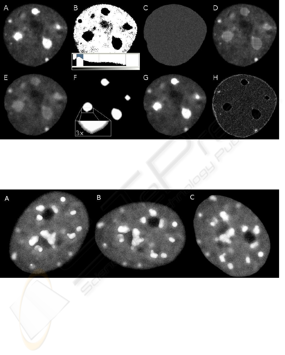
Figure 4: Example of image formation. A) A sample image. B) Its intensity histogram and thresholded image with thresholds

set as shown in the histogram. C) The background ﬁlled with randomly chosen values. D) The sample image with foreground

regions ﬁlled in. E) The same image after the averaging ﬁlter. F) The weights used together with the extended foreground

mask, brighter intensity shows higher weight. G) The artiﬁcial image (the last image in the sequence). H) A map of intensity

differences between A) and G), maximum brightness is at value of 30. Note that the highest errors were due to erroneous

segmentation of the background. All images were enhanced for the purpose of displaying.

Figure 5: Example of 3 frames from image sequence. A) The ﬁrst frame (the last generated). B) The middle frame. C) The

last frame (the ﬁrst generated). All images were enhanced for the purpose of displaying.

ages in the sequence to look more realistic. We made

use of rotation and translation transformations for

global motion (of the entire cell) and only translations

for independent local movements of foreground com-

ponents (selected intracellular structures). The trans-

formations used can be arbitrary, owing to the formal-

ism of the ﬂow ﬁeld, provided they are continuous be-

cause of limitation of both transformation methods.

Seamless overlaying of the foreground was achieved

by the weighted insertion of foreground which im-

proved the robustness to any imprecision in the fore-

ground segmentation. We also made use of local

movements mask which gave us ultimate control over

the independent foreground movements.

We believe that the framework is applicable to

other ﬁelds as well. In some circumstances, image

processing subroutines may differ as well as different

foreground movements may be desired. The require-

ment is that images should be separable into just two

layers and that the background should be reasonably

easy to generate. For instance, in the vehicle control

applications one may meet the requirement: observ-

ICINCO 2007 - International Conference on Informatics in Control, Automation and Robotics

238

Table 1: Similarity comparison from several aspects. The column “Ext.” shows the number of dilations performed on the input

foreground mask beforehand. The upper indices denote whether the foreground regions were simply overlaid

or merged

into the background. A) and B) Comparisons over 2D images. C) Comparison over a 3D image. D) Comparison over the

same 3D image, separate pools of voxel intensities were used for each slice during the formation of the artiﬁcial background.

Ext. Corr.

Avg. diff.

RMS

Corr.

Avg. diff.

RMS

A 0 0.989 3.87 5.13 0.989 3.87 5.12

1 0.989 3.80 5.03 0.989 3.85 5.05

2 0.989 3.73 4.94 0.989 3.82 5.00

3 0.989 3.68 4.90 0.989 3.83 4.98

B 0 0.992 2.76 3.83 0.992 2.77 3.85

1 0.992 2.62 3.69 0.992 2.74 3.75

2 0.993 2.41 3.46 0.992 2.62 3.58

3 0.993 2.33 3.40 0.992 2.64 3.57

C 0 0.980 3.67 4.79 0.980 3.67 4.79

1 0.980 3.73 4.89 0.980 3.81 4.92

2 0.981 3.53 4.69 0.981 3.70 4.77

3 0.981 3.42 4.59 0.981 3.66 4.72

D 0 0.982 3.15 4.16 0.982 3.16 4.17

1 0.983 3.07 4.08 0.982 3.13 4.11

2 0.983 3.00 4.03 0.983 3.11 4.08

3 0.984 2.92 3.96 0.983 3.10 4.05

ing an image of a car on the road can be split into the

car foreground and rather uniform road background.

ACKNOWLEDGEMENTS

The presented work has been supported by the Min-

istry of Education of the Czech Republic (Grants No.

MSM0021622419, LC535 and 2B06052).

REFERENCES

Barron, J. L., Fleet, D. J., and Beauchemin, S. S. (1994).

Performance of optical ﬂow techniques. Int. J. Com-

put. Vision, 12(1):43–77.

Beauchemin, S. S. and Barron, J. L. (1995). The computa-

tion of optical ﬂow. ACM Comput. Surv., 27(3):433–

466.

edras, C. and Shah, M. A. (1995). Motion based recog-

nition: A survey. Image and Vision Computing,

13(2):129–155.

Eils, R. and Athale, C. (2003). Computational imaging in

cell biology. The Journal of Cell Biology, 161:447–

481.

Galvin, B., McCane, B., Novins, K., Mason, D., and Mills,

S. (1998). Recovering motion ﬁelds: An evaluation

of eight optical ﬂow algorithms. In In Proc. of the 9th

British Mach. Vis. Conf. (BMVC ’98), volume 1, pages

195–204.

Gerlich, D., Mattes, J., and Eils, R. (2003). Quantitative

motion analysis and visualization of cellular struc-

tures. Methods, 29(1):3–13.

Horn, B. K. P. and Schunck, B. G. (1981). Determining

optical ﬂow. Artiﬁcial Intelligence, 17:185–203.

Huben

y, J. and Matula, P. (2006). Fast and robust segmen-

tation of low contrast biomedical images. In In Pro-

ceedings of the Sixth IASTED International Confer-

ence VIIP, page 8.

Lehmussola, A., Selinummi, J., Ruusuvuori, P., Niemisto,

A., and Yli-Harja, O. (2005). Simulating ﬂuorescent

microscope images of cell populations. In IEEE En-

gineering in Medicine and Biology 27th Annual Con-

ference, pages 3153–3156.

Lin, T. and Barron, J. (1994). Image reconstruction error

for optical ﬂow. In Vision Interface, pages 73–80.

Saito, T. and Toriwaki, J. I. (1994). New algorithms for Eu-

clidean distance transformations of an n-dimensional

digitized picture with applications. Pattern Recogni-

tion, 27:1551–1565.

Ulman, V. (2005). Mosaicking of high-resolution biomed-

ical images acquired from wide-ﬁeld optical micro-

scope. In EMBEC’05: Proceedings of the 3rd Euro-

pean Medical & Biological Engineering Conference,

volume 11.

Webb, D., Hamilton, M. A., Harkin, G. J., Lawrence, S.,

Camper, A. K., and Lewandowski, Z. (2003). Assess-

ing technician effects when extracting quantities from

microscope images. Journal of Microbiological Meth-

ods, 53(1):97–106.

Young, I. (1996). Quantitative microscopy. IEEE Engineer-

ing in Medicine and Biology Magazine, 15(1):59–66.

Zitov

a, B. and Flusser, J. (2003). Image registration meth-

ods: a survey. IVC, 21(11):977–1000.

ON GENERATING GROUND-TRUTH TIME-LAPSE IMAGE SEQUENCES AND FLOW FIELDS

239