AUTONOMOUS TRACKING SYSTEM FOR AIRPORT LIGHTING

QUALITY CONTROL

J. H. Niblock, K. McMenemy, S. Ferguson and J. X. Peng

School of Electronics, Electrical Engineering and Computer Science, Queen’s University Belfast, United Kingdom

Keywords:

Airport approach lighting, autonomous tracking, grey level assessment.

Abstract:

The central aim of this research is to develop an an autonomous measurement system for assessing the perfor-

mance of an airport lighting pattern. The system improves safety with regard to aircraft landing procedures by

ensuring the airport lighting is properly maintained and conforms to current standards and recommendations

laid down by the International Civil Aviation Organisation (ICAO).

A vision system, mounted in the cockpit of an aircraft, is capable of capturing sequences of airport lighting

images during a normal approach to an aerodrome. These images are post-processed

to determine the grey

level of the approach lighting pattern (ALP). In this paper, two tracking algorithms are presented which can

detect and track individual luminaires throughout the complete image sequence. The effective tracking of

the luminaires is central to the long term goal of this research, which is to assess the performance of the

luminaires’ from the recorded grey level data extracted for each detected luminaire. The two algorithms

presented are the Niblock-McMenemy (NM) feature tracking algorithm has been optimised for the speciﬁc

task of airport lighting and to assess its effectiveness it has been compared to the Kanade-Lucus-Tomasi (KLT)

feature tracking algorithm. In order to validate both algorithms a synthetic 3D model of the ALP is presented.

To further assess the robustness of the algorithms results from an actual approach to a UK aerodrome

are

presented.

The results show that although both KLT and NM feature trackers are both effective in tracking airport lighting

the NM algorithm is better suited to the task due to its reliable grey level information. Limitations, such as the

static window size, of the KLT algorithm result in a lossy grey level data and hence lead to inaccurate results.

Algorithms are being developed for real-time processing

Belfast International Airport

1 INTRODUCTION

A substantial increase in the demand for air trans-

port has resulted in the larger size of aircraft and in-

creased frequency of ﬂights. This requires higher per-

formance and better maintenance of the airport light-

ing pattern (Matsunaga, 1980). One such way of

achieving this is to regularly monitor airport lighting

with the aim of highlighting and repairing any under-

performing luminaires.

Several land based measurement systems such

as the Mobile Airﬁeld Light Monitoring System

(MALMS

) and Photometric Airﬁeld Calibration

http://www.tmsphotometrics.com/

(PAC

) are capable of assessing the performance of

inset runway lighting through the use of light me-

ters and cameras respectively. Typically these sys-

tems work by collecting data as a truck drives over

or past the rows of lighting. However, the major lim-

itation of these systems are that they are incapable of

assessing the performance of the approach lighting

were the luminaires are raised a minimum distance

of 2m above ground level. Thus, this paper proposes

an aerial imaging system that is capable of assessing

the approach lighting during an approach to an aero-

drome.

Milward (Milward, 1976) was the ﬁrst person in

http://www.gsilight.com/ppaclabcombo.htm

317

H. Niblock J., McMenemy K., Ferguson S. and X. Peng J. (2007).

AUTONOMOUS TRACKING SYSTEM FOR AIRPORT LIGHTING QUALITY CONTROL.

In Proceedings of the Second International Conference on Computer Vision Theory and Applications - IU/MTSV, pages 317-324

 SciTePress

1976 to acknowledge the potential of an aerial imag-

ing system in assessing the performance of airport

lighting. With the advance of mobile technology and

external storage devices it is easier and quicker than

ever to process the lighting patterns performance. It

is possible to assess the performance of aerodrome

ground lighting (AGL) using aerial based imaging

techniques (McMenemy and Dodds, 2003). A vision

system is platform mounted, to minimise the effects

of vibration, in the cockpit of an aircraft. During a

normal approach to an aerodrome a video sequence

is captured, approximately 2 minutes in length. The

video is split into its component frames and analysed

off-line. Not all frames are analysed. For the pur-

poses of this paper a subsection of the acquired im-

ages, namely the section including the approach light-

ing pattern (ALP) are used for the performance as-

sessment.

This paper presents two algorithms. The ﬁrst

termed the Niblock-McMenemy (NM) feature track-

ing algorithm has been optimised for the application

of tracking an airport lighting pattern. To place the

algorithm in context, it is compared and contrasted to

the KLT feature tracking algorithm which is seen as

one of the standard algorithms for tracking applica-

tions. Before the autonomous tracking algorithms are

detailed, in the following section, an overview of the

lighting pattern and the vision system are presented.

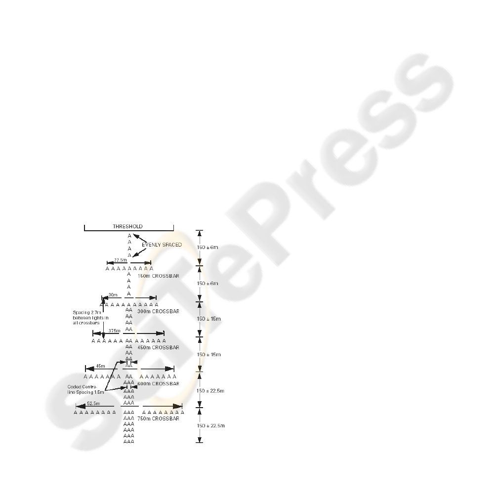
Figure 1: CATI Approach Lighting Pattern.

1.1 Approach Lighting Pattern Layout

Strict guidelines exist for the location and position-

ing of the luminaires. Such standards are docu-

mented in the International Civil Aviation Organisa-

tions (ICAO) Standards and recommended practices

documents (ICAO, 2004).

Milward presents an overview of the standard

Calvert System. This is the standardised lighting sys-

tem used in the UK and Europe. The approach light-

ing system consists of a 900m coded line of white

lights, on the extended centreline of the runway, and

ﬁve crossbars at 150m intervals. The bars decrease in

width towards the runway threshold, lines through the

outer lights of the bars convergingto meet the runway

centreline 300m upwind from the threshold (Milward,

1976). This is illustrated in ﬁgure 1 (ICAO, 2004).

1.2 Vision System Overview

The vision system consists of a monochrome vision

sensor with manual lens mounted on a vacuum based

platform to minimise the effects of vibration. The

vision sensor is connected to an Intel Pentium IV

processor. Controller software acts as an interface be-

tween the processor and the vision sensor. A USB2.0

medium acts as a communications/power mechanism

between computer and vision sensors.

1.3 Autonomous Luminaire Tracking

Tracking has been extended to a number of applica-

tions from video surveillance; medical research and

image reconstruction (Pollefeys and Gool, 1999) to

name a few. This paper is concerned with tracking

lighting performance. To this end a lot of research ex-

ists for street lighting however this paper is concerned

with monitoring an airport ALP. Two tracking algo-

rithms are presented. The ﬁrst algorithm termed the

Niblock-McMenemy (NM) algorithm is introduced in

section 2 and is summarised in ﬁgure 2. This is a fea-

ture extraction algorithm that tracks a series of single

pixels through an image sequence.

The second technique termed the Kanade-Lucus-

Tomasi (KLT) algorithm (Lucas and T.Kanade, 1981)

is a globally recognised feature tracking algorithm

and is introduced in section 3. The KLT method de-

ﬁnes the measure of match between ﬁxed-sized fea-

ture windows in the past and current frame as the sum

of squared intensity differences over the windows.

The displacement is then deﬁned as the one that min-

imises this sum. For small motions, a linearisation of

the image intensities leads to a Newton-Raphson style

minimisation (Tomasi and Kanade, 1991).

Figure 2: NM Tracking Algorithm Overview.

This paper compares and contrasts the NM algo-

rithm with the adapted KLT algorithm. In order to do

this a synthetic model of the approach lighting pattern

(ALP) has been generated (section 4) in order to sim-

ulate a real life approach to an aerodrome. As a means

of measuring the performance of an ALP a measure of

the total grey level of each luminaire is recorded over

the duration of an approach to the aerodrome. This

provides the system with information on each lumi-

naires performance which in turn allows the system to

make a decision on whether or not the lighting pattern

conforms to the relevant standards. Section 5 presents

grey level results obtained from actual images cap-

tured during a real-life approach to a UK aerodrome

These images are used to assess the robustness of the

tracking algorithms and highlight potential improve-

ments. Future work and conclusions are presented in

sections 6 and 7 respectively.

2 NM TRACKING ALGORITHM

This section presents the NM tracking algorithm com-

posed of three states: locking state, tracking state and

the recovery state. The three states are highlighted in

ﬁgure 2.

The authors would like to thank Flight Precision

(http://wwwﬂightprecision.co.uk) for allowing us ﬂight

time whilst performing maintenance work on Belfast Inter-

national Airport’s lighting.

2.1 Locking State

The objective of the locking state is to home in on

the target. The target being the approach lighting pat-

tern. When the target is of acceptable size (McMen-

emy and Dodds, 2003) the imaging system triggers

and starts to acquire data. The video segment is cur-

rently analysed off-line

. A check is performed on

the subsequent image sequence to assess if the image

is skewed and in need of realignment. A line approxi-

mating the horizon is drawn on the ﬁrst image and the

skew angle computed. Using this angle the image is

rotated by the appropriate factor ensuring the rows of

luminaires are in straight lines. The horizon can have

an adverse effect on the extraction process. Stray light

can cause the extraction algorithm to detect too many

luminaires. Therefore, once the horizonhas been used

to de-skew the images the region of interest (ROI) i.e.

the ALP is cropped, making sure to retain the original

positional information.

2.2 Tracking State

Once the target has been identiﬁed the next step is to

extract the relevant foreground information and track

it through the image sequence. The following process

is undertaken to extract, identify and track the lu-

minaires. Each image contains a set of foreground,

bright pixels termed blobs. If the extraction process

were ideal, each detected blob would relate to a single

luminaire in the lighting pattern. The objective of the

extraction process is to highlight the useful informa-

tion, foreground information, from a set of dark pix-

els termed background information or noise. Back-

ground differencing and thresholding techniques are

used to minimise the effects of noise in the image.

Connected Component Analysis (CCA) using 8-

way connectivity(Haralick and Shapiro, 1993) is used

to yield a set of binary points used to segment the im-

age into regions. This process yields a set of smooth

blobs corresponding to each of the moving objects.

The objective of the connected component analysis

is to determine the connected set of components in

an image and assign a distinct label to each pixel in

the same connected component. The number of lu-

minaires (blobs) present depends on the category of

lighting pattern. This information is obtained from

the standards (ICAO, 2004). For the purposes of this

paper a CATI ALP is assumed with a total of 120 ap-

proach luminaires.

It is the long term aim to have an imaging system that

works in real-time. All algorithms are being developed with

this objective in mind.

A center of mass algorithm shown in equation 1

is used to compute the mean x,y coordinate for each

detected blob in the image.

{ ¯x

, ¯y

} =







∑

j∈J

∑

j∈J







(1)

where ¯x

, ¯y

represents the coordinate of the i

blob,

i∈I represents the set of detected blobs’ in the image

and J

represents the set of m

individual pixels that

constitutes the blob.

In a binary image an unlabelled object is assigned

a label based on its (x,y) image location. A scan is

undertaken of the neighbouring objects until all the

blobs have been labelled. The usual notation used to

label the blobs is a set of integers (1...N) where N

corresponds to the number of blobs detected in the

image. The objective of thresholding and image dif-

ferencing is to minimise the probability that noise in

any given image will affect the CCA results. There

are occasions when this is not the case:

1. Inadequate sensor resolution can lead to merging

of luminaires

2. Reﬂections may cause stray noise and ﬂag up

light sources that should not be present in the

ALP

3. Luminaires leaving and entering the ﬁeld of view

of the sensor

4. Occlusions, where a luminaire is obstructed by

an obstacle from the ﬁeld of view of sensor. In

the case of an occlusion the luminaire must be

tracked and only when it has left the screen for

10 consecutive images can it be dropped.

If the expected number of luminaires is not equal to

the actual number of luminaires extracted during the

CCA a recovery state is required, see ﬁgure 2. A

count is kept of blobs that fall out of the FOV of

the sensor. This count is deducted from the expected

number of luminaires to keep the system accurate. de-

tected blobs in the ﬁrst image (120) so that

2.3 Recovery State

This is a correspondence problem, i.e. given a feature

in an image, what is the corresponding feature (i.e.

the projection of the same 3D feature) in the other

image (Pollefeys and Gool, 1999). Let’s assume p

and q to be of the form expressed in equations 2 and

3 respectively.

p = x

(2)

q = x

( f−1)i

(3)

where p is a blob in the current image (f) and q is a

blob in the previous image (f-1) and i denotes the blob

number/id.

For each blob q

in the previous frame, the objec-

tive is to locate the blob p

which is closest to it in the

current frame and assign it the same label. A number

of problem scenarios can arise. This happens when

there is a mismatch between the number of luminaires

in the current frame compared to the previous frame.

Two scenarios can occur:

1. Less luminaires are present in the current frame

2. More luminaires are present in the current frame

In the ﬁrst scenario the 2D Euclidean distance (4)

of each blob in the current frame is computed from

each blob in the previous frame. When a num-

ber of blobs satisfy the Euclidean distance, i.e.

E(p,q) ≤ threshold where threshold is the maximum

displacement a luminaire may shift between consec-

utive images, their grey level and pixel count are

searched to ﬁnd the closest correlation. The resul-

tant blob is matched and the process repeated for

all N blobs in the image frame. If a blob fails to

be matched, i.e. E(p,q) > threshold, it is assigned

a ﬂag ’0’. To compensate for this the CCA re-

sults (luminaireNo, position, greyLevel, pixelCount)

are incremented to accommodate the missing blob

(Gonzalez and Woods, 2004). Once all the blobs in

the current image have been matched the frame num-

ber f is incremented and the process repeated.

E(p,q) =

∑

i=1

− q

)

(4)

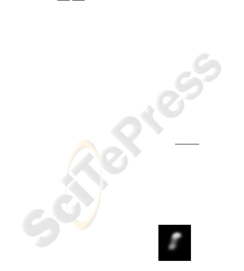
The second scenario is that of having too many

blobs in the current image frame. This is typically

caused by extreme cases of vibration and luminaires

coming back into the ﬁeld of view of the imaging sen-

sor from an occlusion. Figure 3 shows an example

luminaire that appears to consist of two bright spots

with an axon of interconnecting darker pixels. De-

pending on the threshold this blob can be represented

by one/two luminaires. There are two ways of ascer-

Figure 3: The Effects of Vibration on a Single Luminaire.

taining when a luminaire has split into two parts or

components due to vibration:

1. There are too many luminaires present in the

current frame

2. The pixel count for each component is less than

the expected value from the last frame

When the recovery algorithm is called it scans the

grey level comparing the current frame with the pre-

vious frame. At the same time, the pixel count (that

is the number of pixels that constitute a luminaire) is

also compared. When a luminaire splits, the value of

the grey level and the pixel count decreases. Once

the luminaires at fault are identiﬁed, the problem is

rectiﬁed by summing the associated pixel counts and

grey levels together for the problem luminaire. The

problem luminaire still has multiple locations, due to

being split, so a new position is evaluated using equa-

tion 1. The aforementioned CCA results are updated

accordingly, by decrementing the data one element,

so that the effects of vibration are accounted for and

the actual number of luminaires is consistent with that

of the last frame.

This section has introduced the reader to the NM

algorithm and its basic operation. The following sec-

tion introduces the KLT feature tracker algorithm.

3 KLT TRACKING ALGORITHM

This section introduces the theory behind the Kanade-

Lucus-Tomasi (KLT) algorithm before analysing how

it performs on the synthetic airport lighting model

presented in section 4.

As the camera moves, the platform of image in-

tensities change in a complex way. In general, any

function of three variables I(x,y,t), where the space

variables x and y as well as the time variable t are

discrete and suitably bounded, can represent an im-

age sequence. However, images taken at near time

instants are usually strongly related to each other, be-

cause they refer to the same scene taken from only

slightly different viewpoints.

We usually express this correlation by saying that

there are patterns that move in an image stream. For-

mally, this means that the function I(x,y,t) is not ar-

bitrary, but satisﬁes the property shown in equation

I(x, y, t + τ) = I(x− ξ,y− η,t); (5)

where, a later image taken at time t + τ can be ob-

tained by moving every point in the current image,

taken at time t, by a suitable amount. The amount

of motion d = (ξ,η) is called the displacement of the

point x=(x,y) between the time instants t and t+ τ, and

is in general a function of x,y,t and τ (Shi and Tomasi,

1994).

An important problem in ﬁnding the displacement

d of a point from one frame to the next is that a single

pixel cannot be tracked, unless it has very distinctive

brightness with respect to its neighbours. In fact, the

value of the pixel can both change due to noise, and

be confused with adjacent pixels. As a consequence,

it is often hard or impossible to determine where the

pixel went in the subsequent frame, based only on lo-

cal information. Due to these problems the KLT algo-

rithm doesn’t track single pixels but windows of pix-

els and it looks for windows that contain sufﬁcient

texture. Formally, if we redeﬁne J(x) = I(x,y,t+ τ),

and I(x − d) = I(x − ξ,y − η,t), where the time has

been dropped for brevity, our local image model is

represented by equation 6.

J(x) = I(x− d) + n(x), (6)

where n is noise. The displacement vector d is then

chosen so as to minimise the residue error deﬁned by

the double integral over the given window W shown

in equation 7

ε =

[I(x− d) − J(x)]

wdx (7)

In this expression, w is a weighting function. In the

simplest case w could be set to 1. Alternatively, w

could be a Gaussian like function, to emphasise the

central area of the window. This is user deﬁned.

Several methods have been proposed to minimise the

residue in equation 7. This paper assumes the lin-

earisation method used when the displacement d is

much smaller than the window size and is detailed in

(Tomasi and Kanade, 1991).

3.1 Adapting the KLT Algorithm

By default the KLT algorithm accepts a series of

Portable Gray Map (PGM) image ﬁles as the input

ﬁle and outputs a Portable Pixel Map (PPM) results

ﬁle. A number of alterations, ﬁgure 4, were car-

ried out in order to make the airport lighting images,

in either Audio Video Interleave (AVI) or uncom-

pressed bitmap (BMP) format, compatible with the

KLT tracking algorithm. These alterations allow the

KLT algorithm to accept a BMP, AVI or PGM ﬁle

as the input and store the results in a structure, an

AVI video with tracked results superimposed or a se-

quence of PPM image ﬁles with tracked results su-

perimposed. A number of other alterations were per-

formed and are highlighted in later sections.

The next section introduces a virtual model of the

approach lighting pattern used to compare and con-

trast the two tracking algorithms covered in sections

4.1 and 4.2.

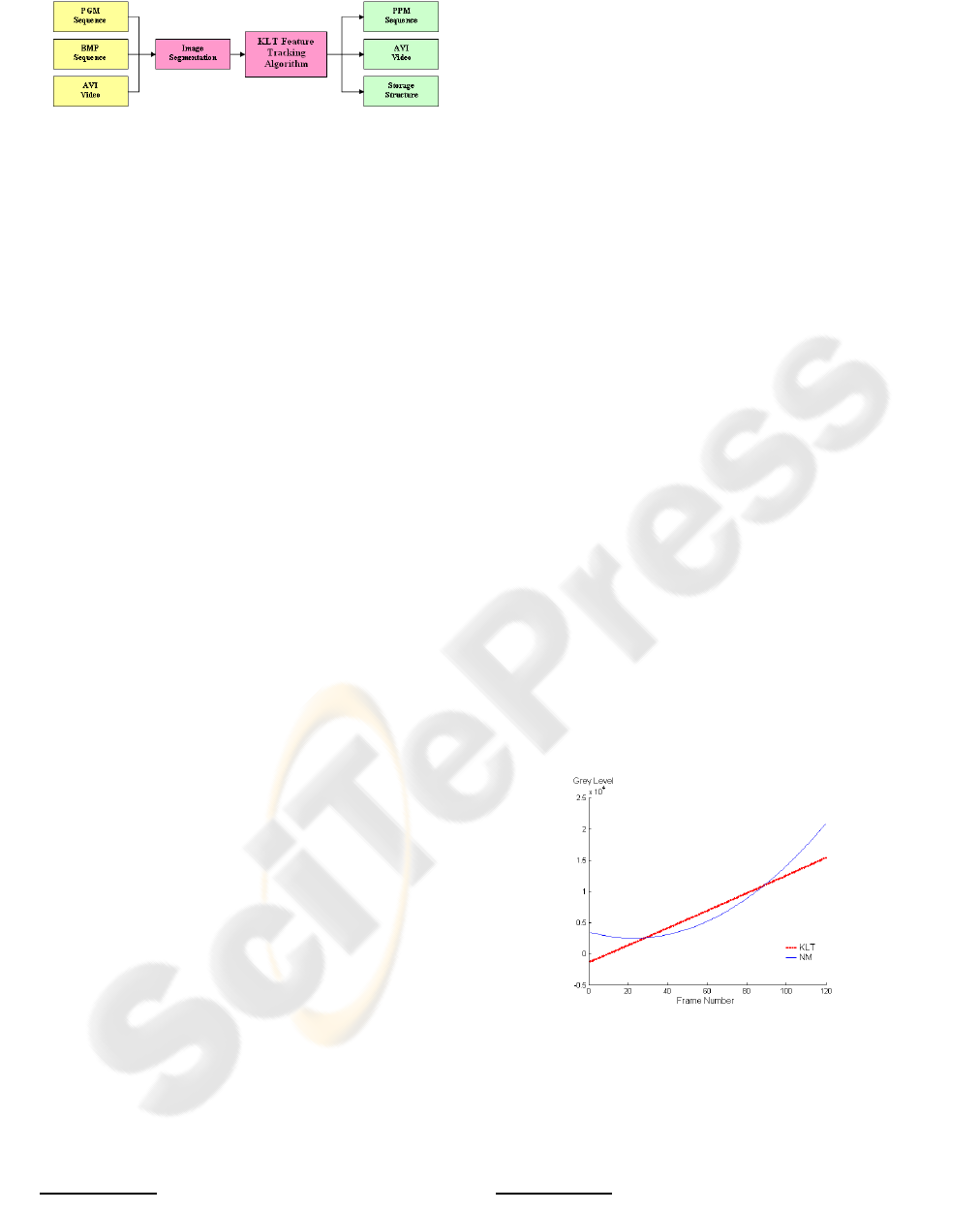
Figure 4: Upgrades to KLT Algorithm.

4 TRACKING VALIDATION

Virtual modelling and scene renderingare particularly

useful in cases where it is not viable to continually

test developed algorithms on a real life model. To aid

testing and comparison of the tracking algorithms a

3D model of the approach airport lighting pattern has

been generated. 2D information taken from Belfast

International Airport is adapted to include luminaire

height information, obtained from the ICAO stan-

dards (ICAO, 2004), and rendered into a 3D model

using OpenFX software

. This model offers a low

cost solution to test the tracking algorithms presented

in this paper and highlight any limitations the algo-

rithms may have. As strict guidelines are enforced on

lighting pattern layout a generic ALP model can be

used to represent any CATI lighting pattern. Three

assumptions are made about the ALP:

1. All luminaires are present in the lighting pattern

2. All luminaires have equal performance

3. No noise exists in the image sequence - such as

horizon, ground and runway markings

4.1 NM Model Response

The model data was tracked using the NM tracking

algorithm outlined in section 2. A complete approach

to the ALP was simulated over 150 images. All lumi-

naires were correctly identiﬁed, labelled and tracked

throughout the image sequence. A relationship exists

between the total grey level and distance. As the air-

craft gets closer to the luminaires, i.e.the frame num-

ber increases, so too does the surface area of each lu-

minaire and hence the total grey level. This is rep-

resented in 5 where a best ﬁt polynomial is used to

represent the grey level data. The grey level informa-

tion for each extracted luminaire will be used, in later

research, to assess the performanceof the luminaires’.

As such it is important that the tracking algorithm is

able to correctly record the grey level information.

The NM algorithm was able to track and record the

grey level of all the luminaires in the lighting pattern

taking a total average time of 355.796 seconds to run,

see table 1.

http://www.openfx.org/

4.2 KLT Model Response

In order to adapt the KLT algorithm two variables are

varied, namely the window size and the number of fea-

tures. When all features are present there is a total

of 120 luminaires in the ALP, therefore the number

of features to track is 120. The second constant is

the window size. For the purposes of this research

this was set to 7x7 pixels. As the effects of noise

have been ignored in the synthetic data due to the sur-

roundings being controlled no further alterations to

the generic KLT algorithm are required.

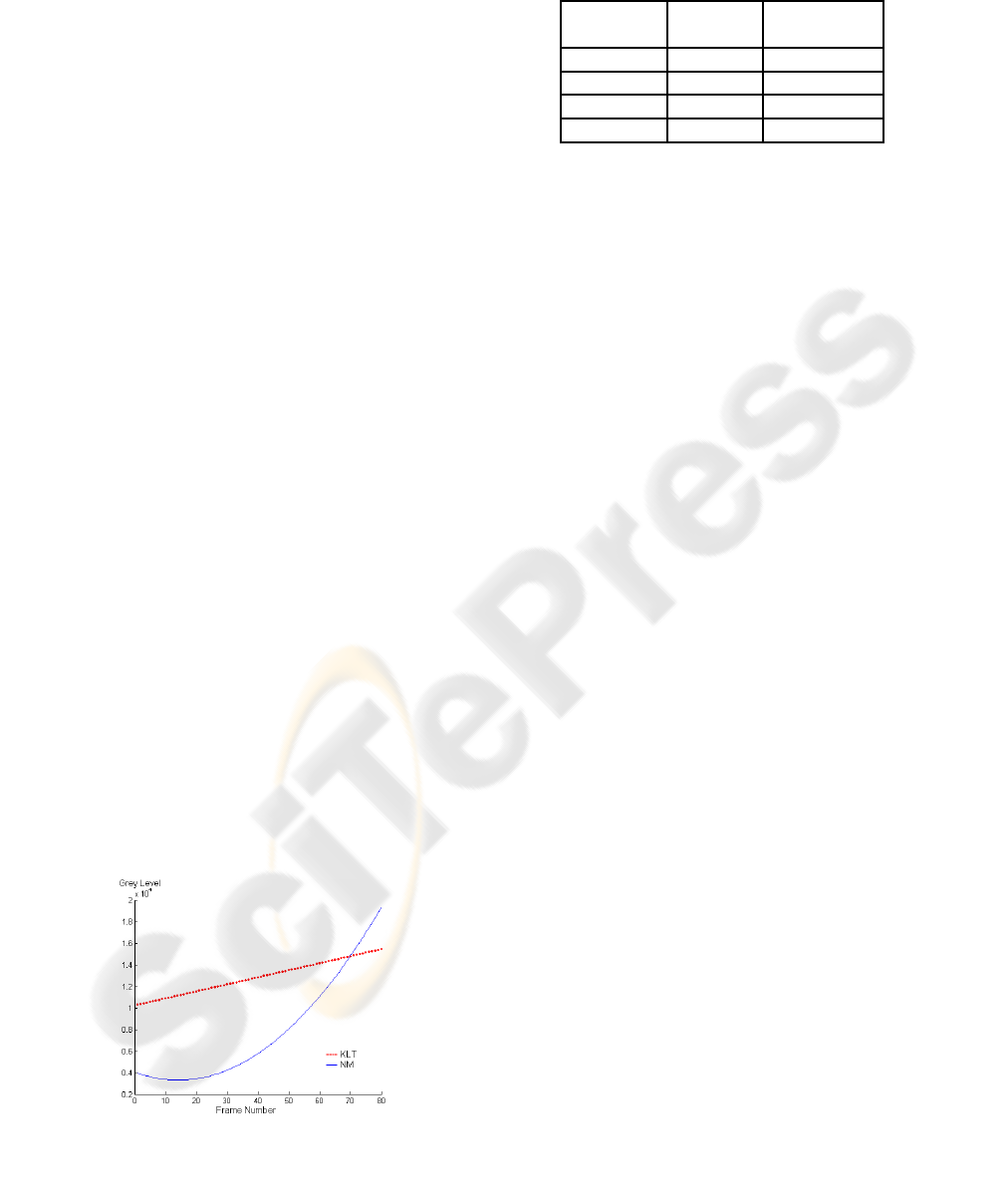
The KLT algorithm took 378.52 seconds to exe-

cute 150 frames, see table 1

. The algorithm performs

well on the ALP outputting a similar trend of increas-

ing grey level to that the NM algorithm. The results

for a random luminaire are presented in ﬁgure 5. A

problem can arise due to the static window size im-

plemented by the KLT algorithm. If a maximum 8-bit

grey level of 220 is used for each pixel (above this

value saturation occurs which is not desirable) then a

window of 7x7 pixels has a maximum grey level of

17380. This is below the top end of the grey level val-

ues obtained in ﬁgures 7 and 8 respectively (as much

as 45000). At the onset of the approach minimal dis-

ruption occurs as the luminaires cover a small num-

ber of pixels. However, as the aircraft gets closer to

the luminaires the luminaires cover a larger number

of pixels (outside the predeﬁned range of the KLT al-

gorithm) and hence the grey level data is termed to be

lossy. In order to avoid this the window size can be

increased. This however has its own problems such as

features being merged as the window size is too large.

For more details see section 6.

Figure 5: Synthetic Grey Level Data Comparison.

All results are averaged over 5 program executions.

5 ACTUAL APPROACH DATA

This section uses actual approach data to further test

the effectiveness of the NM and KLT feature tracking

algorithms. The section has two main aims: To test

the robustness of the tracking algorithms and to as-

sess whether or not the synthetic model is an accurate

representation of an actual approach.

5.1 Sample Results

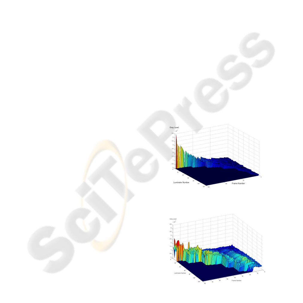
The NM grey level data for a complete approach is

shown in ﬁgure 8. The ﬁrst thing to note is the trend

between the simulated results and the actual results.

Like ﬁgure 7, ﬁgure 8 shows how the luminaires go

from a low grey level (5000) to a high grey level

(30000) as the aircraft gets closer to the luminaires.

For the KLT algorithm a number of alterations

have to be made to the system presented in section

4.2, these additions are detailed in ﬁgure 4. As the ef-

fects of noise, especially the horizon, are more com-

mon in the real images a rectangle function is used to

segment the region of interest (ROI) in the actual im-

ages where the ROI is the ALP. If this step is not im-

plemented false features are sent to the KLT algorithm

rendering the grey level data meaningless. The results

are summarised in table 1. Figure 6 shows how as the

NM algorithm accurately captures the grey level data

above the 17000 mark. In comparison the KLT al-

gorithm tails off losing valuable grey level and hence

performance information. The KLT starts off in frame

one with a grey level of approximately 11000 whereas

the NM algorithm starts at 4000. The luminaire cho-

sen at random was one furthest away from the vi-

sion system. As such the NM algorithm merged it

with neighbouring blobs resulting in multiple under-

performing luminaires and one over-performinglumi-

naire.

Figure 6: Actual Grey Level Data Comparison.

Table 1: NM versus KLT Results for Actual(A) and Syn-

thetic(S) Data.

Algorithm Time/ Extracted

Name Frame(s) Features(%)

KLT(A) 1.90 93

KLT(S) 2.52 95

NM(A) 2.04 98

NM(S) 2.4 98

5.2 Discussion

The NM algorithm has an average execution time of

2.04 seconds/frame. This has a strong correlation

with the execution time of the synthetic model in sec-

tion 4.1. However, as the NM is a point tracker on

occasions mismatches can occur. An example of this

can occur when two luminaires have the same Euclid-

ean distance and similar grey levels. This can lead

to luminaire histories being confused. The KLT al-

gorithm performs well on the actual images. It is

able to successfully extract 93% of the luminaires and

track them through an image sequence. However, it

is clear that if this method is to be used to track the

airport lighting more advanced noise removal tech-

niques, like that shown for the NM algorithm in sec-

tion 2.2, are required to minimise the effects of back-

ground noise.

6 FUTURE WORK

One of the major limitations with the KLT algorithm

is the inaccuracy caused by the static window size. If

the window size is too small this will result in inaccu-

rate grey level information. If the window size is too

large, the luminaires will be merged. For this applica-

tion it is essential that the grey level is computed cor-

rectly. To this end a dynamic window is proposed that

will vary according to the aircraft displacement from

the lighting pattern. The NM algorithm uses CCA

for this purpose. Therefore, if the tracking aspect for

the KLT is merged with the performance assessment

form the NM algorithm the optimum tracking algo-

rithm will be realised. A second limitation of the KLT

algorithm is the effects of background noise. A model

of the background noise can be created and using dif-

ferencing techniques subtracted rom the image data in

order to reduce the effects of noise. As a ﬁnal note,

image tracking is only capable of classifying the lu-

minaires into a pass/fail category. Future work has to

be done into producing performance assessment in-

formation for the ALP.

7 CONCLUSION

Two contributions are presented in this paper. The

ﬁrst is a tracking algorithm that can successfully track

the luminaires in an airport ALP. The second is a tool

for verifying the tracking algorithms without the need

for actual image data.

To satisfy the ﬁrst objective, two tracking algo-

rithms are presented that assess the grey level of lu-

minaires in a CATI airport ALP. Both the NM and

the KLT algorithms are capable of tracking the syn-

thetic and actual approach reliably, with over 90% of

the features being successfully tracked. However, a

limitation of the KLT algorithm was found to be the

static nature of the window size and its vulnerabil-

ity to background noise. The NM algorithm, being

a point tracker, is prone to false matches which can

lead to confused luminaire histories. Therefore, it is

proposed that a combination of the two algorithms be

found for optimum tracking.

The second objective was to assess if the synthetic

model proposed is an accurate model for an approach

to the aerodrome. The results are conclusive. The

model data has a strong correlation with that of the

actual data. This is shown in ﬁgures 7 and 8 respec-

tively. However, research is still required to make the

model more realistic. Accurate correction for noise

has to be realised. This can be done in OpenFX by

adding rain, fog, ground markings and a horizon.

ACKNOWLEDGEMENTS

The authors would like to thank the European Social

Fund (ESF) and the Royal Academy/Society of Engi-

neers for their ﬁnancial backing. The authors would

also like to thank Flight Precision for allowing us

ﬂight time.

REFERENCES

Gonzalez, R. and Woods, R. (2004). Digital Image Process-

ing using Matlab. Pearson Prentice Hall.

Haralick, R. and Shapiro, L. (1993). Computer and Robot

Vision vol. 2. Addison-Wesley Publishing Company

Inc.

ICAO (2004). Aerodrome Design and Operations. Annex

14, Volume 1, Fourth Ed.

Lucas, B. and T.Kanade (1981). An iterative image regis-

tration technique with an application to stereo vision.

In Proc. 7th Int Joint Conference on Artiﬁcial Intelli-

gence, Vancouver, pp.674-679.

Matsunaga, N. (1980). Automatic monitoring system for

the ccr and aerodrome lighting system on airport sys-

tem. In IECI Annual Conference Proceedings (Indus-

trial Electronics and Control Instrumentation Group

of IEEE, p411-416).

McMenemy, K. and Dodds, G. (2003). Calibration and

use of video cameras in the photometric assessment of

aerodrome ground lighting. In The International So-

ciety for Optical Engineers, Electronic Imaging, Vol.

5017, pp. 104-115.

Milward, R. (1976). New approach to airport lighting in-

spection. In Shell Aviation News, Vol. 437, pp26-31.

Pollefeys, M. and Gool, L. V. (1999). Self-calibrated and

metric 3d recognstruction from uncalibrated image se-

quences. In PhD Thesis.

Shi, J. and Tomasi, C. (1994). Good features to track.

In Proceedings of the IEEE Computer Society Con-

ference on Computer Vision and Pattern Recognition,

p593-600.

Tomasi, C. and Kanade, T. (1991). Detection and traking

of point features. In Shape and Motion from Image

Streams: a Factorization Method-Part 3, Technical

Report CMU-CS-91-132.

APPENDIX

Figures 7 and 8 respectively show the grey level data

for an ALP for a synthetic and actual approach.

Figure 7: Synthetic Grey Level Data for NM Algorithm.

Figure 8: Actual Grey Level Data for NM Algorithm.