ACTIVE OBJECT DETECTION

G. de Croon

MICC-IKAT, Universiteit Maastricht, P.O. Box 616, 6200 MD, Maastricht, The Netherlands

Keywords:

Object Detection, Active Vision, Active Scanning, Evolutionary Algorithms.

Abstract:

We investigate an object-detection method that employs active image scanning. The method extracts a local

sample at the current scanning position and maps it to a shifting vector indicating the next scanning position.

The method’s goal is to move the scanning position to an object location, skipping regions in the image that

are unlikely to contain an object. We apply the active object-detection method (AOD-method) to a face-

detection task and compare it with window-sliding object-detection methods, which employ passive scanning.

We conclude that the AOD-method performs at par with these methods, while being computationally less

expensive. In a conservative estimate the AOD-method extracts 45 times fewer local samples, leading to a

50% reduction of computational effort. This reduction is obtained at the expense of application generality.

1 INTRODUCTION

Object detection is the automatic determination of im-

age locations at which instances of a predeﬁned ob-

ject class are present. Numerous methods for object

detection exist (e.g., (Viola and Jones, 2001; Fergus

et al., 2006)), most of which scan a part of the image

at some stage of the object-detection process. Until

now, this scanning is performed in a passive manner:

local image samples extracted during scanning are not

used to guide the scanning process. We mention two

main object-detection approaches that employ passive

scanning here. The window-sliding approach to ob-

ject detection (e.g., (Viola and Jones, 2001)) employs

passive scanning to check for object presence at all

locations of an evenly spaced grid. This approach ex-

tracts a local sample at each grid point and classiﬁes it

either as an object or as a part of the background. The

part-based approach to object detection (e.g., (Fer-

gus et al., 2006)) employs passive scanning to de-

termine interest points in an image. This approach

calculates an interest-value for local samples (such

as entropy of gray-values at multiple scales (Kadir

and Brady, 2001)) at all points of an evenly spaced

grid. At the interest points, the approach extracts new

local samples that are evaluated as belonging to the

object or the background. Although some methods

try to limit the region of the image in which passive

scanning is applied (e.g., (Murphy et al., 2005)), it

remains a computationally expensive and inefﬁcient

scanning method: at each sampling point computa-

tionally costly feature extraction is performed, while

the probability of detecting an object or suitable inter-

est point can be low.

In this article, we investigate an object detec-

tion method that employs active scanning (based on

(de Croon and Postma, 2006)). In active scanning lo-

cal samples are used to guide the scanning process:

at the current scanning position a local image sam-

ple is extracted and mapped to a shifting vector indi-

cating the next scanning position. The method takes

successive samples towards the expected object loca-

tion, while skipping regions unlikely to contain the

object. The goal of active scanning is to save compu-

tational effort, while retaining a good detection per-

formance. In a companion article, we address the

importance of our approach for Embodied Cognitive

Science (de Croon and Postma, 2007). In this article

we focus on the practical applicability in computer

vision. In particular, we verify whether the method

reaches its goal for a face-detection task studied be-

fore in (Kruppa et al., 2003; Cristinacce and Cootes,

2003). We compare the method’s performance and

computational complexity with that of the object de-

tectors (belonging to the window-sliding approach)

employed in the previous studies.

The rest of the paper is organised as follows. In

Section 2, we introduce the object-detection method.

de Croon G. (2007).

ACTIVE OBJECT DETECTION.

In Proceedings of the Second International Conference on Computer Vision Theory and Applications - IU/MTSV, pages 97-103

 SciTePress

Then, in Section 3, we explain our experimental

setup. In Section 4 we analyse the results of the ex-

periments. We draw our conclusions in Section 5.

2 ACTIVE OBJECT-DETECTION

METHOD

The active object-detection method (AOD-method)

scans the image for multiple discrete time steps in or-

der to ﬁnd an object. In our implementation of the

AOD-method this process consists of three phases: (i)

scanning for likely object locations on a coarse scale,

(ii) reﬁning the scanning position on a ﬁne scale, and

(iii) verifying object presence at the last scanning po-

sition with a standard object detector. Both the ﬁrst

and the second phase are executed by an ‘agent’ that

extracts features from local samples, and maps these

features to scanning shifts in the image. We refer to

the agent of the ﬁrst phase as the ‘remote’ agent and

to the agent of the second phase as the ‘near’ agent.

Fe a tu re Ex t ra ct io n

Co ntrolle r

Age nt

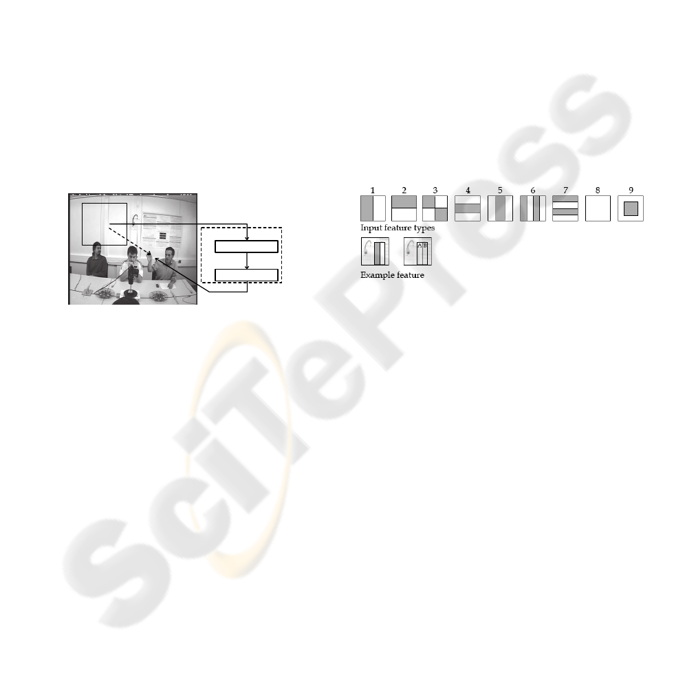
Figure 1: One time step in the scanning process.

Figure 1 illustrates one time step in the scanning

process. At the ﬁrst time step (t = 0) of a ‘run’, the

remote agent takes a local sample at an initial, ran-

dom location in the image (‘x’ in the ﬁgure). The lo-

cal sample consists of the gray-values in the scanning

window. First, the agent extracts features from this

local sample. Then, its controller transforms these

features to a scanning shift in the image (dashed ar-

row) that leads to a new scanning location (‘o’). We

do not allow the scanning window to leave the image.

On the next time step (t = 1), at the new scanning lo-

cation, the process of feature extraction and shifting

is repeated. The sequence of sampling and shifting

continues until t = T, where T is an experimental pa-

rameter. The goal of the remote agent is to center the

local sampling window on an object at t = T. Be-

cause the remote agent does not always succeed in

its goal, we employ a near agent. It starts scanning

at the ﬁnal scanning position of the remote agent and

makes scanning shifts until t = 2T. At t = 2T we ver-

ify object presence at the ﬁnal scanning position with

a standard object detector, such as the one in (Viola

and Jones, 2001).

3 EXPERIMENTAL SETUP

3.1 Agent Implementation

We ﬁrst discuss the feature extraction and then the

controller. We adopt the integral features introduced

in (Viola and Jones, 2001). These features represent

contrasts in mean light intensity between different ar-

eas in an image. The main advantage of these features

is that they can be extracted with very little compu-

tational effort, independent of their scale. Figure 2

shows the types of features that we use in our exper-

iments. We illustrate an example of a feature in the

bottom of Figure 2. The feature is of type 1 and spans

a large part of the right half of the scanning window.

The value of this feature is equal to the mean gray-

value of all pixels in area A minus the mean gray-

value of all pixels in area B. The example feature will

respond to vertical contrasts in the image. Since all

gray-values are in the interval [0, 1], the feature value

is in the interval [−1,1].

Figure 2: Feature types (top) and example feature (bottom).

We extract n features from the sampling window.

They form a vector that serves as input to the con-

troller, which is a completely connected multilayer

feedforward neural network. The network has h hid-

den neurons and o = 2 output neurons, all with a sig-

moid activation function: f(x) = tanh(x). The two

output neurons encode for the scanning shift (∆x,∆y)

in pixels as follows: ∆x = ⌊o

j⌋, ∆y = ⌊o

j⌋. The

constant j represents the maximal displacement in the

image in pixels.

3.2 Evolutionary Algorithm

We employ a ‘µ, λ’ evolutionary algorithm (B

ack,

1996) to select the features and optimise the neu-

ral network weights of both the remote and the near

agent, for the following two reasons. First, an evo-

lutionary algorithm can optimise both the controller

and the feature extraction simultaneously. Second, an

evolutionary algorithm optimises the controller over

the entire chain of samples and actions, from t = 1 to

t = T, enabling the agent to employ non-greedy scan-

ning policies. We ﬁrst evolve the remote agent for

uniformly distributed starting positions, and then the

near agent in the following manner. We measure the

average distance of the evolved remote agent to the

nearest object at t = T in the images of the training

set. Then, we evolve the near agent for positions that

are normally distributed with as mean an object posi-

tion and as standard deviation the measured average

distance at t = T.

We split evolution in two by evolving both the fea-

tures and the neural network weights in the ﬁrst half,

and evolving only the neural network weights in the

second half. Evolution starts with a population of λ

different agents. An agent is represented by a vector

of real values (doubles), referred to as the genome.

In this genome, each feature is represented by ﬁve

values, one for the type and four for the two coor-

dinates inside the scanning window. Each neural net-

work weight is represented by one value. We evalu-

ate the performance of each agent on the task by let-

ting it perform R runs per training image, each of T

time steps. The ﬁtness function we use in the ﬁrst half

of evolution is: f

(a) = (1− distance(a))+ recall(a),

where distance(a) ∈ [0,1] is the normalised distance

between the agent’s scanning position at t = T and

its nearest object, averaged over all training images

and runs. The term recall(a) is the average propor-

tion of objects that is detected per image by an en-

semble of R runs of the agent a. An object is detected

if the scanning position is on the object. When all

agents have been evaluated, we test the best agent

on the validation set. In addition, we select the µ

agents with highest ﬁtness values to form a new gen-

eration. Each selected agent has λ/µ offspring. To

produce offspring, there is a p

probability that one-

point cross-over occurs with another selected agent.

Furthermore, the genes of the new agent are mutated

with probability p

mut

. The process of ﬁtness eval-

uation and procreation continues for G generations.

As mentioned, we stop evolving the features at G/2.

In addition, we set p

to 0, since cross-over might

be disruptive for the optimisation of neural network

weights (Yao, 1999). Moreover, we gradually dimin-

ish p

mut

. Finally, we also change the ﬁtness function

to f

(a) = recall(a). At the end of evolution, we

select the agent that has the highest weighted sum of

its ﬁtness on the training set and validation set (ac-

cording to the set sizes) to prevent overﬁtting.

The near agent is evolved in exactly the same man-

ner as the remote agent, except for the different start-

ing positions (close to the objects) and the ﬁtness

function: g(a) = (1 − distance(a)) + precision(a),

which does not change at G/2. precision(a) is the

proportion of runs R of the near agent that detect ob-

jects at the end of the run. The goal of the near agent is

to reﬁne the scanning position reached by the remote

agent, by detecting the nearest object and approaching

its center as much as possible.

The third phase of the AOD-method, the object

detector that veriﬁes object-presence at the last scan-

ning position, is not evolved, but trained according to

the training scheme in (Viola and Jones, 2001).

3.3 Face-detection Task

We apply the AOD-method to a face-detection task

that is publicly available. We use the FGNET video

sequence (http://www-prima.inrialpes.fr/FGnet/

which contains video sequences of a meeting room,

recorded from two different cameras. For our

experiments we used the joint set of images from

both cameras (’Cam1’ and ’Cam2’) in the ﬁrst

scene (’ScenA’). The set consists of 794 images of

720 × 576 pixels, which we convert to gray-scale.

We use the labelling that is available online, in which

only the faces with two visible eyes are labelled.

For evolution, we divide the image set in two parts:

half of the images is used for testing and half of the

images for evolution. The images for evolution are

divided in a training set (80%), and a validation set

(20%). We perform a two-folded test to obtain our

results, and run one evolution per fold.

3.4 Experimental Settings

Here we provide the settings for our experiments. The

maximal scanning shift j is equal to half the image

width for the remote agent, and equal to one third of

the image width for the near agent. The scanning win-

dow is a square with sides equal to one third of the

image width for the remote agent, and one fourth of

the image width for the near agent. The number of

time steps per agent is T = 5, and the number of runs

per image R is 20. We use n = 10 features that are ex-

tracted from the sampling window. We set the num-

ber of hidden neurons h of the controller to n/2 = 5,

while the number of output neurons o is 2. We set the

evolutionary parameters as follows: λ = 100, µ = 25,

G = 300, p

mut

= 0.04, and p

= 0.5.

4 RESULTS

4.1 Behaviour of the Evolved Agents

In this subsection, we give insight into the scanning

behaviour of the remote and near agents evolved on

the ﬁrst fold (their behaviour on the second fold is

similar). Figure 3 shows ten independent runs of the

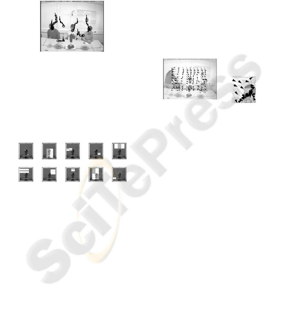
remote agent. At t = 0, all runs are initialised at ran-

dom positions in the image. The method then succes-

sively takes samples and makes scanning shifts (ar-

rows). At the end of scanning (t = T) seven out of

ten runs have reached an object location. The ﬁnal

locations of the runs are indicated with circles.

Figure 3: Ten independent runs of the remote agent.

The ﬁgure indicates that the evolutionary algo-

rithm found suitable features and neural network

weights for the remote agent. Figure 4 shows the ten

evolved features inside the scanning window (white

box) centered in the image (‘x’ indicating the scan-

ning location) and the types, sizes and locations of

the features. Although it is not straightforward to in-

terpret the features, we can see that it contains both

coarse contextual features (e.g., features 2 and 9) and

more detailed object-related features (e.g., features 3,

5, and 8).

Feature 1 Feature 2 Feature 3 Feature 4 Feature 5

Feature 6 Feature 7 Feature 8 Feature 9 Feature 10

Figure 4: The ten evolved features of the remote agent.

The controller maps these features to scanning

shifts that approach the target objects. In the left part

of Figure 5, we illustrate the function of the remote

agent’s controller by taking local samples at a ﬁxed

grid, and visualising both the direction and size of the

scanning shifts. The controller deﬁnes a gradient map

on the image that has attractors at persons and at heads

in particular. Few of the arrows go upwards. This

property of the behaviour is mainly due to two factors.

First, the prior distribution of object locations is such

that faces usually occur in the lower half of images.

Second, the ﬁtness function of the remote agent pro-

motes recall. Since the agent is evaluated on the en-

semble of R runs, it can ‘loose’ a few runs in the bot-

tom of the image as long as the other runs are success-

ful. This raises the issue whether the method exploits

more than the prior distribution of face-locations. The

AOD-method cannot exploit this prior distribution di-

rectly, since it only uses visual features. However, it

can exploit it indirectly for samples that contain little

information on the object position. Indeed, in the face

images, the remote agent seems to have a preference

for moving down instead of up. However, the method

can move up if the features contain enough informa-

tion (see the arrows under the face of the standing per-

son). In addition, in (de Croon and Postma, 2006), a

different version of the AOD-method performed well

on a task of license-plate detection in which there was

no strong prior distribution of object locations. In

the right part of Figure 5, we show the scanning be-

haviour of the near agent, close to an object. The near

agent considerably improves performance on the de-

tection task, as will be shown in the next subsection.

Figure 5: Remote agent’s actions at different locations (left)

and near agent’s actions close to a face (right).

4.2 Performance Comparison

For a possible computational efﬁciency of the AOD-

method to be relevant, the active object-detection

method must at least have a sufﬁcient performance.

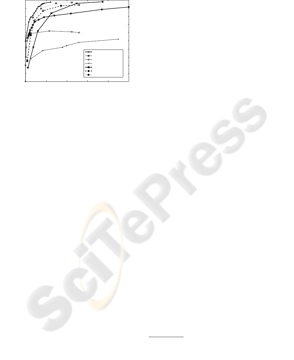
Figure 6 shows an FROC-plot of our experimental

results (square markers, thick lines), for the remote

agent alone (solid line), the remote and near agent in

sequence (dashed line), and the sequential agent fol-

lowed by the ﬁrst stage of a Viola and Jones-detector

trained according to the training scheme in (Viola and

Jones, 2001) (dotted line, only based on the ﬁrst test-

ing fold). We created these FROC-curves by varying

the number of runs: R = 1,3,5,10,20, and 30. In ad-

dition, the ﬁgure shows the results on the FGNET im-

age set from other studies, made by varying the classi-

ﬁer’s threshold: from (Cristinacce and Cootes, 2003)

(thin lines), of a Fr

oba-K

ullbeck detector (Fr

oba and

ullbeck, 2002) (‘+’-markers) and a Viola and Jones

detector (Viola and Jones, 2001) (‘o’-markers). It

also shows the results of two Viola and Jones de-

tectors trained on a separate image set and tested on

the FGNET set (Kruppa et al., 2003) (thick lines).

The ﬁrst of these detectors attempts to detect face re-

gions in the image, as the detectors in (Cristinacce

and Cootes, 2003) (‘o’-markers). The second of these

detectors attempts to detect a face by including a re-

gion around the face, including head and shoulders

(‘x’-markers).

0 5 10 15 20 25

0.1

0.2

0.3

0.4

0.5

0.6

0.7

0.8

0.9

FPs / image

Recall

Kruppa et al. − context

Kruppa et al. − V&J

Cristinacce & Cootes − V&J

Cristinacce & Cootes − F−K

AOD: first agent

AOD: sequential

AOD: seq + V&J

Figure 6: FROC-plot of the object-detection methods.

Figure 6 shows that the AOD-method outperforms

the window-sliding approaches that did not include

a face’s context for detection rates higher than 65%.

Detecting faces without considering context is difﬁ-

cult in the FGNET video-sequence, because the ap-

pearance of a face can change considerably from im-

age to image (Cristinacce and Cootes, 2003). How-

ever, the context of a face (such as head and shoul-

ders) is rather ﬁxed. This is why approaches that

exploit this context (such as (Kruppa et al., 2003))

have a more robust performance. The active object-

detection method exploits context even to a greater

extent than in (Kruppa et al., 2003) that only includes

a small area around the object.

The difference between the Viola and Jones-

classiﬁer used in (Cristinacce and Cootes, 2003) and

(Kruppa et al., 2003) can be explained by at least three

factors: the different training set, different parame-

ter settings of the training method for the Viola and

Jones-classiﬁer, and a different labeling. In (Kruppa

et al., 2003) proﬁle faces are also labeled, while such

faces are not labeled in the labeling available online.

Small differences between the experiments aside, the

results show that the AOD-method performs at par

with other existing object detection methods on the

FGNET face-detection task.

4.3 Computational Efﬁciency

4.3.1 General Comparison

The computational costs C of a window-sliding ap-

proach (WS) and an active object-detection approach

(AOD) can be expressed as:

= G

+Cl) + P (1)

AOD

= R(2T)(F

AOD

+Ct) + R(F

+Cl) + P (2)

The variables G

and G

are the number of horizon-

tal and vertical grid points, respectively. Furthermore,

is the number of operations necessary for fea-

ture extraction in the window-sliding approach, Cl for

the classiﬁer, and P for preprocessing. For the AOD-

approach, R is the number of independent runs and 2T

the number of time steps at which local samples are

used for scanning shifts. F

AOD

is the number of oper-

ations necessary for feature extraction, and Ct for the

controller that maps the features to scanning shifts.

R(F

+Cl) is for verifying object-presence at the ﬁ-

nal scanning position.

The AOD-approach is computationally more ef-

ﬁcient than the window-sliding approach. The main

reason for this is that the AOD-approach extracts

far fewer local samples, i.e., (R(2T) + R) ≪ G

while its feature extraction and controller do not cost

much more than the feature extraction and classiﬁer

of the window-sliding approach. For example, in the

FGNET task a window-sliding approach that veriﬁes

object presence at every point of a grid with a step

size of two pixels will extract 335 × 248 = 83,080

local samples (based on the image size, the average

face size of 50 × 80 pixels, and the largest step size

mentioned in (Viola and Jones, 2001)). In contrast,

the AOD-method extracts R(2T +1) = 20×11 = 220

local samples (sequential agent in combination with

a classiﬁer). Under these conditions, the window-

sliding approach extracts 377.6 times more local sam-

ples than the AOD-method

4.3.2 Estimate of Computational Effort

We estimate the computational effort of both methods

for the face-detection task, expressed in a number of

operations. We make a conservative estimate for the

window-sliding method, the Viola and Jones detec-

tor (Viola and Jones, 2001). Importantly, we make

the conservative assumption that G

= G

= 100,

which implies step sizes of ∆x ≈ 7 and ∆y ≈ 5 in the

FGNET images. As a result, the AOD-method ex-

tracts 45 times fewer local samples. In our estimate

of the Viola and Jones detector, we base ourselves on

the research in (Cristinacce and Cootes, 2003; Kruppa

et al., 2003; Viola and Jones, 2001). We estimate the

remaining variables in equation 1 and 2 as follows:

• F

= 64,F

AOD

= 80: In (Viola and Jones, 2001), the

computational cost of feature extractions was expressed

in array references. The features in Figure 2 require

from 4 to 12 references, with as average ≈ 8 references.

The average number of features extracted per scanning

Note that taking into account different scales of ob-

ject detection would imply a new multiplication factor for

the computational costs, which is disadvantageous for the

window-sliding approach.

location was mentioned to be 8 in (Viola and Jones,

2001), while it is 10 for the AOD-method.

• Cl = 9,Ct = 94: The classiﬁer of the window-sliding

approach makes a linear combination of the features

and compares this to a threshold, and therefore we esti-

mate its cost at the average number of features extracted

plus one: 8+ 1 = 9. In the neural network of the AOD-

method, each hidden and output neuron computes a lin-

ear combination of its inputs and puts the result into

the activation function: Ct = h(n+ 1) + o(h+ n + 1) +

(h+ o) = 94. The ﬁrst two terms represent the compu-

tational costs for the linear combinations made in the

hidden and output neurons, respectively. The last term,

(h+ o), represents the cost for the activation functions.

• P = 414,720: Both methods need to calculate an ‘inte-

gral image’ (see (Viola and Jones, 2001)) for their sub-

sequent feature extractions. The computational cost of

the calculation of the integral image is a pass through

all pixels of the image, being 414,720 pixels for the

720× 576 images.

These estimates lead to C

= 1,144, 720 and

AOD

= 450,980: the application of active scanning

roughly results in a reduction of 50% of the computa-

tional effort. Note that the calculation of the integral

image constitutes the main part of the computational

costs for the AOD-method. The low number of sam-

ples of the AOD-method opens up possibilities for the

real-time application of features that are in themselves

more costly per sample than integral features, but that

require no detailed preprocessing of the entire image.

4.4 Application Generality

The advantages of the AOD-method come at the ex-

pense of application generality. Namely, they rely on

the exploitation of the steady properties of an object’s

context. If these properties are present in the test im-

ages, the method is still able to detect objects. For ex-

ample, Figure 7 shows how the remote agent behaves

if it is applied to photos taken in our own ofﬁce (10 in-

dependent runs of the remote agent per image). Each

scanning shift is represented by an arrow, while the

last scanning position has a circle. The run of the re-

mote agent is followed by the ﬁrst stage of a Viola and

Jones classiﬁer, where the runs shown in black belong

to runs for which the last scanning position was clas-

siﬁed as an object position. In both images the in-

dependent runs cluster at the heads, since the ofﬁce

walls are relatively uncluttered (with an occasional

poster) as in the FGNET video-sequence. However,

if the exploited contextual properties are not present

(as in many outdoor images) detection performance

degrades considerably. The question is how limiting

this loss of generality is. Findings on the human vi-

sual system (Henderson, 2003) suggest that this limi-

tation may be relieved by extending the AOD-method,

so that it applies different scanning policies to differ-

ent visual scenes.

Figure 7: Generalisation of the evolved method.

5 CONCLUSION

We conclude that the AOD-method meets its goal

on the FGNET face-detection task: it performs at

par with existing object-detection methods, while be-

ing computationally more efﬁcient. In a conservative

estimate the active object-detection method extracts

45 times fewer local samples than a window-sliding

method, leading to a 50% reduction of the computa-

tional effort. The advantages of the AOD-method de-

rive from the exploitation of an object’s context and

come at the cost of application generality.

REFERENCES

ack, T. (1996). Evolutionary Algorithms in Theory and

Practice. Oxford University Press, New York, Oxford.

Cristinacce, D. and Cootes, T. (2003). A comparison of

two real-time face detection methods. In 4

IEEE In-

ternational Workshop on Performance Evaluation of

Tracking and Surveillance, pages 1–8.

de Croon, G. and Postma, E. O. (2006). Active object detec-

tion. In Belgian-Dutch AI Conference, BNAIC 2006,

Namur, Belgium.

de Croon, G. and Postma, E. O. (2007). Sensory-motor

coordination in object detection. In First IEEE Sym-

posium on Artiﬁcial Life.

Fergus, R., Perona, P., and Zisserman, A. (in press - 2006).

Weakly supervised scale-invariant learning of models

for visual recognition. International Journal of Com-

puter Vision.

oba, B. and K

ullbeck, C. (2002). Robust face detection

at video frame rate based on edge orientation features.

In 5

international conference on automatic face and

gesture recognition 2002, pages 342–347.

Henderson, J. M. (2003). Human gaze control during real-

world scene perception. TRENDS in Cognitive Sci-

ences, 7(11).

Kadir, T. and Brady, M. (2001). Scale, saliency and im-

age description. International Journal of Computer

Vision, 45(2):83–105.

Kruppa, H., Castrillon-Santana, M., and Schiele, B. (2003).

Fast and robust face ﬁnding via local context. In Joint

IEEE International Workshop on Visual Surveillance

and Performance Evaluation of Tracking and Surveil-

lance (VS-PETS’03), Nice, France.

Murphy, K., Torralba, A., Eaton, D., and Freeman, W.

(2005). Object detection and localization using lo-

cal and global features. In Sicily workshop on object

recognition. Lecture Notes in Computer Science.

Viola, P. and Jones, M. J. (2001). Robust real-time object

detection. Cambridge Research Laboratory, Technical

Report Series.

Yao, X. (1999). Evolving artiﬁcial neural networks. Pro-

ceedings of the IEEE, 87:1423 – 1447.