ROBUST APPEARANCE MATCHING WITH FILTERED

COMPONENT ANALYSIS

Fernando De la Torre, Alvaro Collet, Jeffrey F. Cohn and Takeo Kanade

Robotics Institute, Carnegie Mellon University, Pittsburgh, USA

Keywords:

Appearance Models, principal component analysis, Multi-band representation, learning ﬁlters.

Abstract:

Appearance Models (AM) are commonly used to model appearance and shape variation of objects in images.

In particular, they have proven useful to detection, tracking, and synthesis of people’s faces from video. While

AM have numerous advantages relative to alternative approaches, they have at least two important drawbacks.

First, they are especially prone to local minima in ﬁtting; this problem becomes increasingly problematic as

the number of parameters to estimate grows. Second, often few if any of the local minima correspond to

the correct location of the model error. To address these problems, we propose Filtered Component Analysis

(FCA), an extension of traditional Principal Component Analysis (PCA). FCA learns an optimal set of ﬁlters

with which to build a multi-band representation of the object. FCA representations were found to be more

robust than either grayscale or Gabor ﬁlters to problems of local minima. The effectiveness and robustness of

the proposed algorithm is demonstrated in both synthetic and real data.

1 INTRODUCTION

Component Analysis (CA) methods such as Principal

Component Analysis (PCA) have been widely applied

in visual, graphics, and signal processing tasks over

the last two decades. PCA is a key learning compo-

nent of Appearance Models (AM). AM have proven

especially powerful for face tracking and synthesis

relative to alternative approaches (e.g. optical ﬂow)

(Blanz and Vetter, 1999; Matthews and Baker, 2004;

Cootes and Taylor, 2001b; de la Torre and Black,

2003; Black and Jepson, 1998).

In applications such as face detection and track-

ing, the goal is to search for a minimum residual be-

tween the image and the model across rigid (e.g. ro-

tation and translation) and non-rigid parameters. For

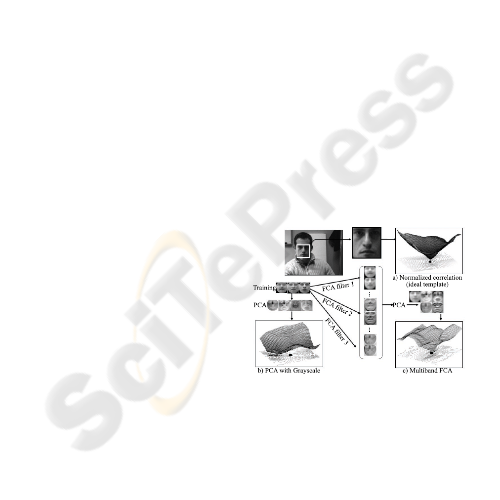
instance, consider ﬁg. 1, in which a face has been

placed in an arbitrary image. In ﬁg. 1.a, we plot

the normalized correlation surface error between the

ideal template (face) and the image in a 40 ×40 patch

centered in the middle of the face. This surface error

has nice local properties: it has just one well deﬁned

global minimum that corresponds to the expected lo-

cation of the face. However, if we learn a generic PCA

a) Normalized correlation

(ideal template)

FCA filter 1

FCA filter 2

FCA filter 3

PCA

c) Multiband FCAb) PCA with Grayscale

Training

PCA

Figure 1: a). Normalized correlation error surface of the

image with the face in a 40 ×40 patch. b) Error function

with a generic graylevel appearance model. The black dot

denotes the optimal position of the face. c) Error function

of a multiband learned representation. The location of the

face corresponds to the minimum of the function.

model of the facial appearance variation from training

data and try to locate the face again, two undesirable

effects may occur. First, the location of the optimal

207

De la Torre F., Collet A., F. Cohn J. and Kanade T. (2007).

ROBUST APPEARANCE MATCHING WITH FILTERED COMPONENT ANALYSIS.

In Proceedings of the Second International Conference on Computer Vision Theory and Applications - IFP/IA, pages 207-212

 SciTePress

parameter (translation) fails to correspond to the lo-

cation of the face (delineated by the the black dot in

the ﬁgure), see ﬁg. (1.b). Second, many local minima

may be found. Even if a gradient descent algorithm

begins close to the correct solution, the occurrence of

local minima is likely to divert convergence from the

desired solution.

The aim of this paper is to explore the use of a new

technique, Filtered Component Analysis (FCA). FCA

learns a multiband representation of the image that re-

duces the number of local minima and improves gen-

eralization relative to PCA. Fig. (1.c) shows the main

goal of the paper. By building a multiband representa-

tion with FCA, we are able to locate the minimum in

the right location (black dot) and eliminate most local

minima close to the optimal one.

2 PREVIOUS WORK

This section reviews work on subspace tracking and

the role of representation in subspace analysis.

2.1 Subspace Detection and Tracking

Subspace trackers build the object’s appearance/shape

representation from the PCA of a set of training sam-

ples. Let d

∈ℜ

d×1

(see notation

) be the i sample of

a training set D ∈ ℜ

d×n

and B ∈ ℜ

d×k

the ﬁrst k prin-

cipal components. B contains the directions of maxi-

mum variation of the data. The principal components

maximize max

∑

i=1

||B

= ||B

B||

, with the

constraint B

B = I. The columns of B form an ortho-

normal basis that spans the principal subspace. If the

effective rank of D is much less than d, we can ap-

proximate the column space of D with k << d princi-

pal components. The data d

can be approximated as

a linear combination of the principal components as

≈Bc

where c

= B

are the coefﬁcients obtained

by projecting the training data onto the principal sub-

space.

Once the model has been learned (i.e. B is

known), tracking is achieved by ﬁnding the para-

meters a of the geometric transformation f(x, a) that

Bold capital letters denote a matrix D, bold lower-case

letters a column vector d. d

represents the j column of the

matrix D. d

i j

denotes the scalar in the row i and column

j of the matrix D and the scalar i-th element of a column

vector d

. All non-bold letters will represent variables of

scalar nature. ||x||

√

x designates Euclidean norm of

x. The vec(D) operator transforms D ∈ ℜ

d×n

into an dn-

dimensional vector by stacking the columns. ◦ denotes the

Hadamard or point-wise product. ⊗ denotes convolution.

∈ ℜ

k×1

is a vector of ones. I

∈ ℜ

k×k

is the identity.

aligns the data w.r.t. the subspace. Given an image d

subspace trackers or detectors ﬁnd a and c

that min-

imize: min

||d

(f(x, a)) −Bc

(or some normal-

ized error). In the case of an afﬁne transformation,

f(x, a) =









x −x

y −y



where

a = (a

, a

) are the afﬁne parameters and

x = (x

, y

, ···, x

, y

) is a vector containing the coor-

dinates of the pixels to track. If a = (a

, a

) is just

translation, the search can be done efﬁciently over

the whole image using the Fast Fourier Transform

(FFT). For a = (a

= a

, a

= a

), that is, for simi-

larity transformation, the search also can be done ef-

ﬁciently in the log-polar representation of the image

with the FFT.

2.2 Representation in Subspace

Analysis

Most work on AM uses some sort of normalized

graylevel to build the representation. However, re-

gions of graylevel values can suffer from large am-

biguities, camera noise, and changes in illumination.

More robust representation can be achieved by local

combination of pixels through ﬁltering. Filtering of

the visual array is a key element of the primate visual

system (Rao and Ballard, 1995).

Representations for subspace recognition were ex-

plored by Bischof et al. (Bischof et al., 2004). In

the training stage, they built a subspace by ﬁlter-

ing the PCA-graylevel basis with steerable ﬁlters. In

the recognition phase, they ﬁltered the test images

and performed robust matching, obtaining improved

recognition performance over graylevel. Cootes et. al

(Cootes and Taylor, 2001a) found that a non-linear

representation of edge structure could improve the

performance of model subspace matching and recog-

nition. De la Torre et al. (de la Torre et al., 2000)

found that subspace tracking was improved by using

a multiband representation created by ﬁltering the im-

ages with a set of Gaussian ﬁlters and its derivatives.

Our work differs in several aspects from previous

work. First, we explicitly learn an optimal set of spa-

tial ﬁlters adapted to the object of interest rather than

using hand-picked ones. Once the ﬁlters are learned,

we build a multiband representation of the image that

has improved error surfaces with which to ﬁt AM. We

evaluate quantitatively the properties of the error sur-

faces and show how FCA outperforms current meth-

ods in appearance based detection.

VISAPP 2007 - International Conference on Computer Vision Theory and Applications

208

3 FILTERED COMPONENT

ANALYSIS

Many component analysis methods (PCA, LDA, etc)

build data models based on the second order statistics

(covariance matrices) of the signal. In particular, PCA

ﬁnds a linear transformation that decorrelates the data

by exploiting the correlation across samples. PCA

models the correlation across pixels of different im-

ages, but not the spatial statistics within each of the

images. In this section, we propose Filtered Compo-

nent Analysis (FCA) that learns a bank of orthogonal

ﬁlters that decorrelate the spatial statistics of a set of

images. Once the FCA ﬁlters are learned, we build a

multi-band representation that generalizes better and

is more robust to different types of noise.

3.1 Learning Spatial Correlation

Previous research (de la Torre et al., 2000; Bischof

et al., 2004; Cootes and Taylor, 2001a) has shown

the importance of representation in AM. However, re-

searchers have used hand-picked ﬁlters to represent

the signal. Instead, FCA will learn a set of orthog-

onal spatial ﬁlters optimal for variance preservation.

Variance preservation of image spatial statistics is a

realistic assumption to build a generative model for

detection or tracking appearance.

Given a set of training images, D

d×n

, our aim is

to model the spatial statistics of the signal by learning

the ﬁlter F that minimizes:

(F, µ

µ) = min

F,µ

∑

i=1

||d

⊗F −µ

µ||

(1)

Recall that ⊗ denotes convolution, and µ

µ =

∑

i=1

⊗F is the mean of the ﬁltered signal. If µ

is known, the optimal F can be achieved by solving:

Avec(F) = b A =

∑

i=1

∑

(x,y)

b =

∑

i=1

∑

(x,y)

◦d

(x,y)

(2)

where (x, y) is the domain where the convolution is

valid and d

(x,y)

is a patch of the ﬁlter size ( f

, f

)

centered at the coordinates (x, y). The matrix A can

be computed efﬁciently in space or frequency from

the autocorrelation function of d

. Analogously, b is

estimated from the cross-correlation between d

and

µ. Alternatively, one could use the integral image

(Lewis, 1995) to efﬁciently compute eq. 2.

Without imposing any constraints on the ﬁlter co-

efﬁcients, the optimal solution of eq. 1 is given by

µ = 0 and F = 0 (although an iterative algorithm will

rarely converge to this solution). To avoid this trivial

solution, we impose that the sum of squared coefﬁ-

cients is 1, i.e. vec(F)

vec(F) = 1. The latter con-

straint can be elegantly solved by noticing that the

convolution is a linear operator, and , eq. 2 can be

rewritten as:

(F) = min

∑

i=1

||(d

−µ

) ⊗F||

(3)

where µ

∑

i=1

is the sample mean. Now

Eq. 3 can be solved by ﬁnding the eigenvec-

tor with smallest eigenvalue of A =

∑

i=1

∑

(x,y)

−

)

(x,y)

−µ

)

(x,y)

(see eq. 2).

3.2 Learning a Multiband

Representation

In this section, we will build a multiband represen-

tation of the signal that preserves most spatial corre-

lation among a given training set. In particular, we

will ﬁnd a set of ﬁlters F

1, ···,F

that decorrelate the

spatial statistics of the image and are orthogonal to

each other. Observe that FCA is analogous to PCA

but now rather than decorrelating the signal with the

covariance of the data, we decorrelate the spatial sta-

tistics.

In our particular tracking application, we are inter-

ested in ﬁnding a set of ﬁlters that preserve the spatial

statistics of the object of interest and has minimal re-

sponse to background. This ﬁlter set can be obtained

by maximizing E

F CA

1, ···,F

F CA

∑

f =1

∑

i=1

||d

⊗F

−λ

∑

j=1

||d

⊗F

(4)

where d

denotes the j

sample of the background.

Let T = [vec(F

) vec(F

) ··· vec(F

)] be a matrix

of all the vectorized ﬁlters, the ﬁlters should satisfy

T = I

F×F

. After making the derivatives with re-

spect to F

, it can be shown that the optimal solutions

satisﬁes the following eigenvalue problem:

max

1, ···,F

∑

i=1

||(A −λBα)vec(F

)||

(5)

A =

∑

i=1

∑

(x,y)

α =

max(A)

max(B)

B =

∑

j=1

∑

(x,y)

s.t. vec(F

)

vec(F

) = 0 ∀i 6= j and

vec(F

)

vec(F

) = 1 ∀i

If λ is large, the set of ﬁlters will predominantly can-

cel the background. If λ is small the ﬁlters will be

adapted to the object.With λ close to one the ﬁlters

will achieve trade-off between modeling the signal

(i.e object) and removing the background. Typically

ROBUST APPEARANCE MATCHING WITH FILTERED COMPONENT ANALYSIS

209

0 ≤ λ ≤ 2. α is an artiﬁcially introduced parameter

that normalizes the energies of A and B.

The solution of eq. 5 is given by the leading eigen-

vectors of (A −λαB). At this point, it is interesting to

consider again the analogy with PCA. PCA will ﬁnd

the leading eigenvectors of

∑

i=1

whereas FCA

will ﬁnd the leading eigenvectors (assuming λ = 0)

A =

∑

i=1

∑

(x,y)

. While PCA ﬁnds the di-

rections of maximum variation of the covariance ma-

trix, FCA ﬁnds the directions of maximum variation

of the sum of all overlapping patches.

Figure 2: a) Training images of faces and background. b)

FCA ﬁlters for λ = 0, λ = 1 and size 11 ×11.

Fig. (2.a) shows many examples of faces and

background patches. Fig.(2.b) shows the set of FCA

ﬁlters for λ = 0 and λ = 1 for size 11 ×11. Observe

that the ﬁrst FCA ﬁlter is an average ﬁlter, and the

other ﬁlters are differential ﬁlters at different orienta-

tions and scales.

3.3 Multiband Subspace Detection

In subspace detection, PCA is computed from a set of

training images. After the training stage, the goal is to

detect the object of interest over different orientation,

scales and translations. If the scale and orientation is

known, dectection can be achieved ﬁnding the trans-

lational parameters a = (a

, a

) that minimize:

= min

||d

(x + a) −Bc

||d

(x + a)||

(6)

Evaluating eq. 6 at each location (x, y) can be com-

putationally expensive. For a particular position (x, y)

computing the coefﬁcients (i.e. c

) is equivalent to

correlating the image with each basis of subspace B,

and stacking all values for each pixel. For large re-

gions, this correlation is performed efﬁciently in the

frequency domain using the Fast Fourier Transform

(FFT) (i.e. C

= b

I = IFFT (FFT (b

) ◦FFT (I))).

Similarly, the local energy term, ||d

(x + a)||

, can

be computed efﬁciently using the convolution in the

space or frequency domain. Alternatively, these ex-

pressions can be computed efﬁciently using the inte-

gral image (Lewis, 1995).

In multiband tracking, we represent an image as

a concatenation of ﬁltered images. For a particular

image d

and a set of ﬁlters (F

, ···, F

), there are

several ways to modify eq. 6:

∑

f =1

||d

⊗F

−B

||d

⊗F

(7)

∑

f =1

||d

⊗F

−B

||d

⊗F

(8)

Parameters β

are the eigenvalues of (A −λαB), ob-

tained by FCA. E

ﬁlters the training images and

builds PCA based on the set of stacked ﬁltered im-

ages. E

computes an independent PCA for each rep-

resentation such that the coefﬁcients for each image

are uncoupled (i.e. c

differs for each ﬁlter).

4 EXPERIMENTS

To test the validity of our approach, we have per-

formed several sets of experiments in face detection

and facial feature tracking. The ﬁrst set of experi-

ments consists on detecting a face embedded in an

arbitrary image (see ﬁg. 1) using a generic model. In

the second set, we test the ability of FCA to improve

tracking in Active Appearance Models (Cootes and

Taylor, 2001b; Blanz and Vetter, 1999; Matthews and

Baker, 2004; de la Torre et al., 2000).

In all experiments a generic face model was built

from 150 subjects from the IBM ViaVoice AV data-

base (Neti et al., 2000), after aligning the data with

Procrustes Analysis(Cootes and Taylor, 2001b). Once

the FCA ﬁlters are learned, a multi-band represen-

tation is built for each of the 150 images, and PCA

is computed retaining 80% of the total energy. For

comparison purposes, multi-band PCA is also done

for other representations (e.g. Gabor, graylevel and

derivatives. In the experiments, we consider Gabor

Filters because of the good results reported by other

researchers in the area. In addition, these ﬁlters have

been shown to possess optimal localization proper-

ties in both spatial and frequency domain and thus are

well suited for tracking problems.

4.1 Understanding FCA

In order to compute FCA 150 subjects are selected

randomly from the IBM database. We also extract

2000 random patches from several images of the IBM

that do not contain faces. Using these training sam-

ples, we learn FCA ﬁlters at 5 different scales (3 ×3,

5 ×5, 7 ×7, 9×9 and 11×11 pixels), using eq. 5 for

different λ values.

VISAPP 2007 - International Conference on Computer Vision Theory and Applications

210

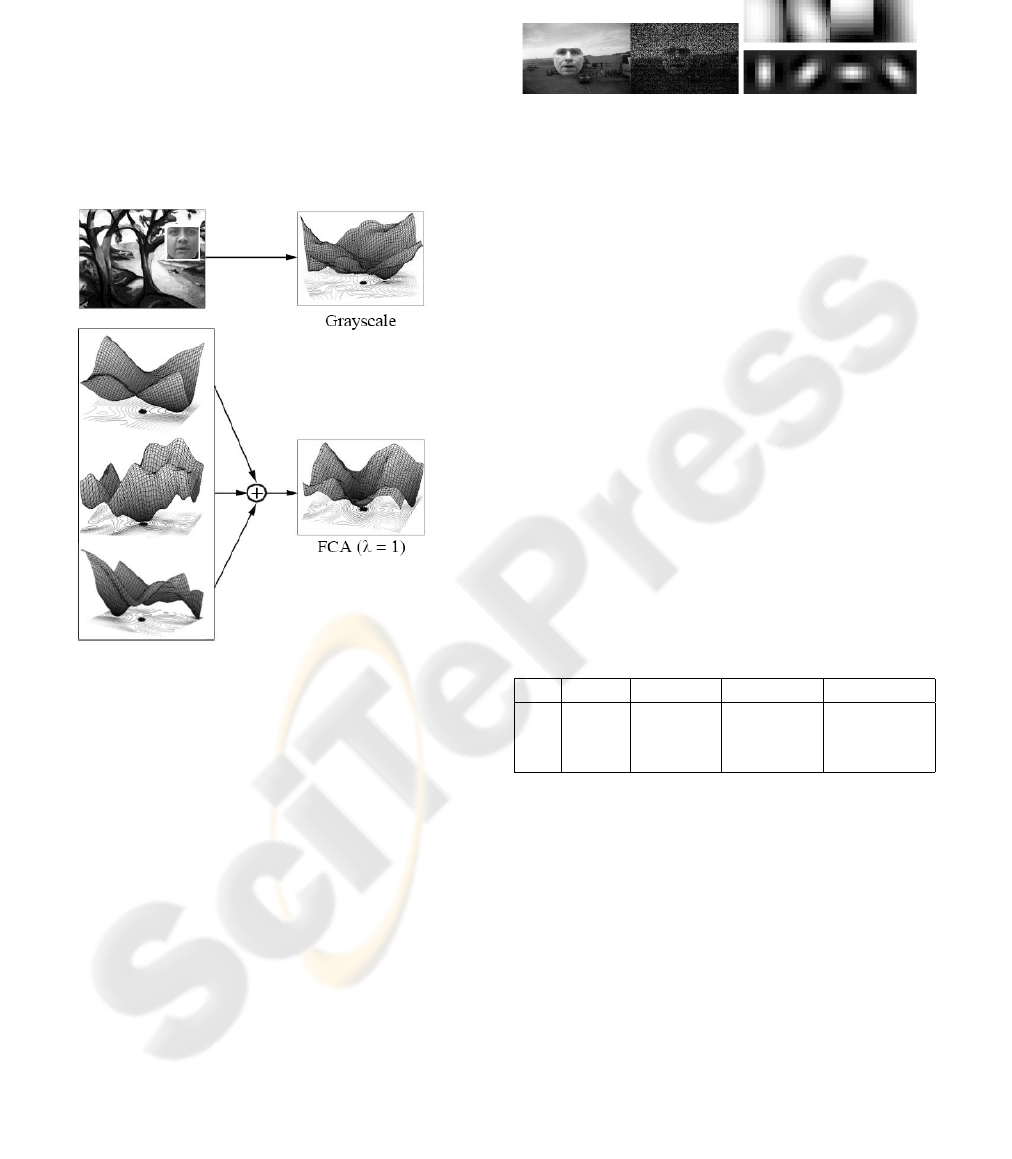
Given a new face image not present in the train-

ing set, we embedded it in a bigger background im-

age (see ﬁg. 3). Then, we efﬁciently search over all

translations looking for a minimum of the subspace

model. Fig. 3 shows an example of the error surface

for each of the FCA bands, in comparison with the

error surfaces from normalized graylevel. As it can

be observed, Graylevel representation has several lo-

cal minima and the global minimum is misplaced. On

the other hand, the sum of the three FCA bands pro-

duces an error surface with a correctly-placed global

minimum.

Figure 3: Error surfaces for graylevel and each of the bands

for FCA.

4.2 Robustness to Noise/Illumination

This ﬁrst experiment is designed to test the robust-

ness of FCA to noise and varying illumination condi-

tions. A subset of 100 subjects from the IBM data-

base (not in the training set) are randomly chosen and

embedded in background images. Then, random im-

pulsional noise is added (see ﬁg. 4.a) and the error

in each location is efﬁciently computed (the orien-

tation and scale is known). To quantitatively com-

pare each ﬁlterbank, 3 different surface error statis-

tics have been calculated. Given a patch of 100 ×100

pixels around the optimal location of the face (which

is known beforehand), we compute the following sta-

tistics: 1) distance between the global minimum and

the face center, 2) distance between the correct mini-

mum and closest local minimum, 3) Amount of local

minima. The amount of local minima in an error sur-

face is calculated by counting those pixels with sign

change in x and y derivatives and positive values in

the second derivatives.

Figure 4: a) Original image and test image with added im-

pulsional noise. b) FCA(11,4) and Gabor (8,4).

Table 1 shows the average results for the described

error statistics for three representations: a set of four

11 ×11 pixels FCA ﬁlters (see ﬁg. 4.a), the best-

performing 11 ×11 pixels Gabor ﬁlter (see ﬁg. 4.b)

and the normalized graylevel. In all our experiments,

we report the results of the set of Gabor ﬁlters that

performs the best over several scales. A global mini-

mum is said to be correct if it falls within a region of

3 ×3 pixels around the theoretical minimum. All the

representations have similar accuracy; however, the

amount of local minima is very high in the grayscale,

and both grayscale and Gabor fail to provide a sufﬁ-

ciently high global-closest minimum margin in com-

parison with FCA ﬁlters. These results are quite sta-

ble across spatial domains of the FCA ﬁlter sets and

have therefore been omitted in the interest of space.

Table 1: Experiments on noisy data. Statistics: (1) Per-

centage of correct global minimum. (2) distance between

correct and closest local minimum. (3) Average number of

local minima.

gray FCA

λ=0

FCA

λ=0.5

Gabor(8,4)

(1) 98 99 99 99

(2) 9.73 24.36 24.03 19.01

(3) 30.06 1.45 1.49 2.46

In the next experiment we test the robustness of

FCA to illumination changes. We take 4 images un-

der varying illumination conditions (see ﬁg. 5) for 30

subjects from the PIE database(Sim et al., 2002) (to-

tal 120 images). We embedded this face into an image

and compute the error surfaces. Results from this ex-

periment can be seen in table 2. In this case, FCA

clearly outperforms any other technique in all three

statistics of the error function. The accuracy is higher

than grayscale and Gabor by 33% and 12% resp.,

while keeping the closest minimum 25.37% pixels

further away and the density of local minima is the

lowest one. It is worth noting that the best-performing

ﬁlters have been FCA

λ=0

(no background). Fig. 6

shows the error surface for a particular subject; as we

can observe, the properties of FCA are more desirable

ROBUST APPEARANCE MATCHING WITH FILTERED COMPONENT ANALYSIS

211

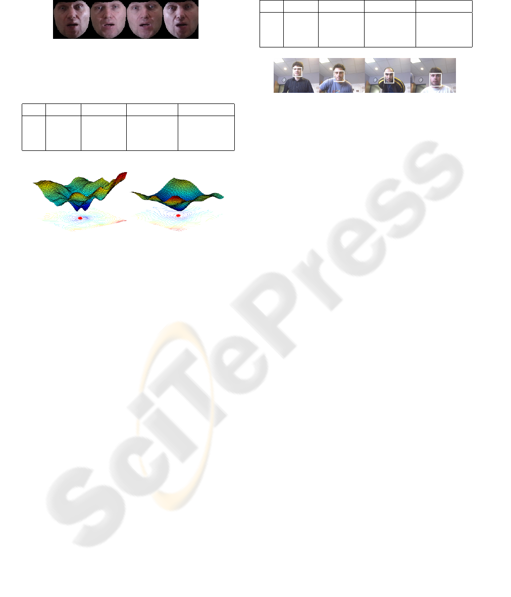
than graylevel or Gabor ﬁlters in terms of location and

density of local minima.

Figure 5: Changes in illumination on the PIE database.

Table 2: Experiments on illumination.(1),(2),(3) see table1.

gray FCA

λ=0

FCA

λ=0.5

Gabor(8,4)

(1) 41 74 73 62

(2) 14.59 26.37 26.04 19.68

(3) 3.28 1.4 1.41 1.92

Figure 6: Error surface for graylevel and FC A

λ=0

(11, 4).

The last experiment of this section explores FCA

performance on images taken in the lab. 10 images

have been collected in the lab (see Fig. 7) with an

inexpensive webcam, and roughly selecting the same

scale manually. Table 3 shows the detection results

of this experiment. As we can see FCA consistently

outperforms other representations that included Ga-

bor and graylevel in all metrics.

5 CONCLUSIONS AND FUTURE

WORK

In this paper, we have proposed FCA to build a multi-

band representation of the image to achieve more

robust ﬁtting and detection with appearance mod-

els. FCA outperforms Gabor, oriented pair ﬁlters and

graylevel representations. Additionally, we have in-

troduced quantitative metrics for evaluating the error

surface. FCA has shown promising results, however

future work should consider the use of different con-

straints for the ﬁlters (e.g. vec(F)

×f

= 1). Also,

it will be worth to explore the use of some recent non-

linear ﬁlters.

Acknowledgements The work was partially sup-

ported by National Institute of Justice award 2005-IJ-

CX-K067 and NIMH grant. Thanks to Iain Matthews

and Simon Lucey for helpful discussions and com-

ments.

Table 3: Experiments on images taken in the lab.(1), (2), (3)

see table 1.

gray FCA

λ=0

FCA

λ=0.5

Gabor(8,4)

(1) 20 80 80 70

(2) 15.71 18.05 25.52 13.53

(3) 2 2 1.2 2.4

Figure 7: Some test images.

REFERENCES

Bischof, H., Wildenauer, H., and Leonardis, A. (2004). Il-

lumination insensitive recognition using eigenspaces.

Computer Vision and Image Understanding, 1(95):86

– 104.

Black, M. J. and Jepson, A. D. (1998). Eigentracking:

Robust matching and tracking of objects using view-

based representation. International Journal of Com-

puter Vision, 26(1):63–84.

Blanz, V. and Vetter, T. (1999). A morphable model for the

synthesis of 3d faces. In SIGGRAPH.

Cootes, T. and Taylor, C. (2001a). On representing edge

structure for model matching. In CVPR.

Cootes, T. F. and Taylor, C. J. (2001b). Statistical

models of appearance for computer vision. In

http://www.isbe.man.ac.uk/bim/refs.html.

de la Torre, F. and Black, M. J. (2003). Robust parame-

terized component analysis: theory and applications

to 2d facial appearance models. Computer Vision and

Image Understanding, 91:53 – 71.

de la Torre, F., Vitri

a, J., Radeva, P., and Melench

on, J.

(2000). Eigenﬁltering for ﬂexible eigentracking. In In-

ternational Conference on Pattern Recognition, pages

1118–1121.

Lewis, J. P. (1995). Fast normalized cross-correlation. In

Vision Interface.

Matthews, I. and Baker, S. (2004). Active appearance mod-

els revisited. International Journal of Computer Vi-

sion, 60(2):135–164.

Neti, C., Potamianos, G., Luettin, J., Matthews, I., Glotin,

H., Vergyri, D., Sison, J., Mashari, A., and Zhou,

J. (2000). Audio-visual speech recognition. Tech-

nical Report WS00AVSR, Johns Hopkins University,

CLSP.

Rao, R. and Ballard, D. (1995). An active vision architec-

ture based on iconic representations. Artiﬁcial Intelli-

gence, 12:441–444.

Sim, T., Baker, S., and Bsat, M. (2002). The cmu pose,

illumination, and expression (pie) database. In IEEE

Conference on Automatic Face and Gesture Recogni-

tion.

VISAPP 2007 - International Conference on Computer Vision Theory and Applications

212