REAL-TIME ADAPTIVE POINT SPLATTING FOR NOISY POINT

CLOUDS

Rosen Diankov* and Ruzena Bajcsy

Dept. of Electrical Engineering and Computer Science

University of California, Berkeley, USA

Keywords:

Hardware rendering point-clouds.

Abstract:

Regular point splatting methods have a lot of problems when used on noisy data from stereo algorithms. Just

a few unﬁltered outliers, depth discontinuities, and holes can destroy the whole rendered image. We present a

new multi-pass splatting method on GPU hardware called Adaptive Point Splatting (APS) to render noisy point

clouds. By taking advantage of image processing algorithms on the GPU, APS dynamically ﬁlls holes and

reduces depth discontinuities without loss of image sharpness. Since APS does not require any preprocessing

on the CPU and does all its work on the GPU, it works in real-time with linear complexity in the number of

points in the scene. We show experimental results on Teleimmersion stereo data produced by approximately

forty cameras.

1 INTRODUCTION

Vision based applications that extract and display 3D

information from the real world are becoming perva-

sive due to the large number of stereo vision packages

available. The 3D information can be used to store

and view virtual reality performances so that view-

ers are free to choose the viewpoint of the scene. A

much more exciting topic called teleimmersion is to

use the 3D information as a form of real-time com-

munication between people at remote locations. In

both these cases, users expect image quality that is in-

distinguishable from reality. However, teleimmersion

requires ﬁltering and displaying the 3D information at

real-time speeds whereas in viewing performances of-

ﬂine, the 3D information can be preprocessed before

hand, so real-time ﬁltering is not an issue. We con-

centrate on the teleimmersion case where the 3D in-

formation is in the form of point clouds computed by

stereo vision. Stereo algorithms produce very coarse

point clouds with a lot of information missing due to

occlusions and lighting conditions. Even if stereo al-

gorithms could compute perfect depths with no out-

liers, the low resolution from the image will be appar-

ent once the user gets close to the surfaces.

Research in the past has tackled point cloud

rendering and ﬁltering from several different direc-

tions. One popular method called point splatting

represents each point as a small gaussian distribu-

tion. By summing up and thresholding these distri-

butions in image space, the algorithm produces very

smooth images (Elliptical Weighted Average Splat-

ting (L. Ren and Zwicker, 2002) and (H. Pﬁster and

Bross, 2000)). Other algorithms represent the neigh-

borhood of each point by patches (Kalaiah and Varsh-

ney, 2001). (Levoy et al., 2000) and (R. Pajarola,

2004) cover the case where the point clouds are com-

posed of millions of points and the CPU and GPU

have to be synchronized together. There has been

a lot of work in converting point clouds to mesh

data (R Kolluri and O’Brien, 2004) using triangula-

tion based methods. Since there are usually people

in teleimmersion scenes, researchers have ﬁt skele-

tons to the point cloud data (Remondino, 2006) and

(Lien and Bajcsy, 2006). The display component

just uses the skeleton to deform a prior model of an

avatar. But one reason for choosing to work with

point clouds instead of meshes is that point cloud ren-

dering is much more efﬁcient than mesh rendering,

and there has been work done in reducing meshes to

point clouds(Stamminger and Drettakis, 2001). The

ﬁltering and reconstruction step in most of these algo-

228

Diankov R. and Bajcsy R. (2007).

REAL-TIME ADAPTIVE POINT SPLATTING FOR NOISY POINT CLOUDS.

In Proceedings of the Second International Conference on Computer Graphics Theory and Applications - GM/R, pages 228-234

DOI: 10.5220/0002078602280234

 SciTePress

rithms is inherently slow and is usually done ofﬂine.

The real-time performance is usually attributed to the

rendering component. Instead of ﬁtting surfaces to

this data in order to remove outliers and ﬁll holes, we

ﬁlter the point clouds directly on the GPU with no

processing.

The Adaptive Point Splatting algorithm most

closely resembles Elliptical Weighted Average Splat-

ting (L. Ren and Zwicker, 2002) in that it does all

ﬁltering on the GPU in image space. In EWA, if a

point cloud was computed by densely sampling from

a 3D model without adding any noise to the point po-

sitions, the ﬁnal point rendering would look just as

sharp as the surface rendering. The intuition behind

the algorithm is that each point represents a probabil-

ity distribution of its color in 3D space. When the

point is rendered, its color distribution is projected

in the image plane. Then all the distributions of all

points are combined and normalized to form the ﬁ-

nal image. If the combined probability is low for any

pixel, that pixel is discarded. Different depths of the

points are taken care of by ﬁrst computing the depth

of the nearest points to the camera for the whole im-

age. For a given pixel, only points within a certain dis-

tance to the nearest depth contribute to the ﬁnal pixel’s

color. It is in the ﬁnal combination steps that EWA

and other point splatting algorithms break down with

noisy point clouds. The reasons will be explained in

Section 2.

An ideal rendering algorithm needs to do three

operations to the point clouds: remove outliers, ﬁll

holes, and smooth the colors on the surface while

maintaining sharpness. Any type of CPU preprocess-

ing like detecting outliers or ﬁlling holes will never

run in real-time if there are more than 50,000 points.

While hierarchical processing can speed up the as-

ymptotic time, it will not work because it takes a sig-

niﬁcant amount of time to organize the data in the

right structures before real work can be done on it.

Organizing the data in volumetric structures, might be

faster. However, a large amount of memory is needed

to maintain even a 1000x1000x1000 cube; resolution

is obviously poor. Even ignoring the time issue, it is

still not clear how to ﬁll holes with these data struc-

tures. Without strong prior information, it is impos-

sible to ﬁt surfaces to arbitrary 3D point clouds in

real-time in order to ﬁgure out if a hole is present

or not, but holes become pretty clear when looking

at the rendered data in 2D. Since the three operations

only require analysis of the local space around each

point, they can be massively parallelized. Hence, the

approach we take is to use modern GPUs to do all

necessary processing in the image space (Figure 1).

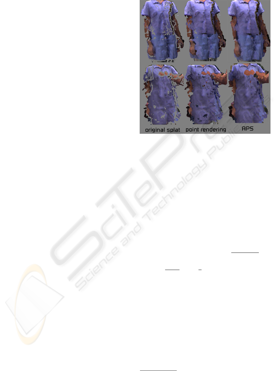
Figure 1: An example comparing the output of previously

proposed splatting algorithms (left) with the current pro-

posed APS method (right). Note that the original point

cloud (middle) is pretty noisy and some information can-

not be recovered at all.

2 POINT SPLATTING REVIEW

Let a point cloud consist of N points {X

} with colors

} and deﬁne a simple multivariate gaussian distri-

bution around each point with covariance {Σ

}. Then

the color C(X) at any point X in the 3D space is de-

ﬁned by

C(X ) =

∑

(X)

∑

(X)

(1)

(X) ∝

|Σ

0.5

exp{−

(X − X

)

−1

(X − X

)} (2)

Here, the probability that the point belongs to

solid space is given by P(X) =

∑

(X). Applying

a simple threshold to P(X) and tracing out the result-

ing surface by an algorithm like Marching Cubes will

generate a geometric surface; however, this method is

slow and cannot be done easily using the GPU only.

Fortunately, most of the work can be ported to the

2D projection space (L. Ren and Zwicker, 2002). Let

∗

be the projection

of Σ

, and ¯x

by the projection

of X

. Then for any point x in the image, the color

can be computed in the same way as in Equation 1.

The advantage is that an explicit surface doesn’t need

The projection of a multivariate gaussian distribution is

again gaussian.

REAL-TIME ADAPTIVE POINT SPLATTING FOR NOISY POINT CLOUDS

229

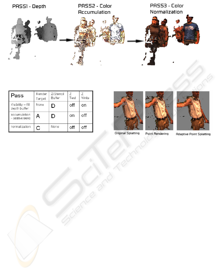
Figure 2: The original splatting method uses 3 passes: the ﬁrst pass computes the depth buffer, the second pass renders the

points that only pass this depth buffer, the third pass normalizes the accumulated colors.

Figure 3: GPU render states for the 3-pass splat algorithm.

to be computed, the disadvantage is that the depth in-

formation gets lost and points that project to the same

pixel but have different depths can interfere with each

other. To partially solve this, EWA uses a 3-pass al-

gorithm on the point clouds (Figure 2). To simulate

a probability surface, each point is represented by a

simple quad whose texture coordinates are used to ex-

tract the probability from its projected gaussian dis-

tribution. The quads can be oriented to always face

the camera, or can be given a static orientation if the

surface normal is known apriori. There are various

ways to compute a gaussian probability on the GPU:

a simple texture can be used as a lookup table, or the

probability can be computed directly in the GPU pixel

shaders by applying Equation 1. We use the texture

mapping method because it is faster and much easier

to get working.

The ﬁrst pass computes the depths of all the near-

est points, so color information is not needed. The

second pass only renders points that are close to the

previously computed depth buffer. The probabili-

ties and colors are combined with additive blending.

The third pass normalizes each color with respect to

the probability and performs the thresholding so that

points with low probabilities are discarded. See Fig-

ure 3 for a description of the GPU state during these

Figure 4: Artifacts occur with the original splatting method

when there are depth discontinuities in the su rface.

passes.

The problem with this simple approach is that

points don’t get ﬁltered and depth discontinuities

cause artifacts (Figure 4). The reason is beacuse the

nearer pixels modify the depth buffer regardless of

what the accumulated probability will be. During

the second pass, only the front pixels are allowed to

be rendered. The third pass sees the low accumu-

lated probability and discards the pixel without con-

sidering pixels on the next nearest layer. This prob-

lem can be easily solved by employing an approach

similar to depth peeling (Everitt, 2001). Depth peel-

ing is an algorithm that can dynamically segment the

view-dependent depth layers on the GPU. In the case

of splatting, if the front layer yields low probabili-

ties, then the next nearest layer will be considered

for rendering. Holes still remain a problem and can-

not be ﬁlled easily with the traditional point splatting

method. To reduce holes, the gaussian variance can

be increased or the cutoff threshold can be decreased

so that fewer points are rejected; however, the image

will get blurry and halos around surfaces will appear.

Also, outliers will be rendered as big splats on the

image. The outlier problem can be solved by decreas-

ing the variance or increasing the cutoff threshold,

but obviously that will introduce holes. Clearly there

GRAPP 2007 - International Conference on Computer Graphics Theory and Applications

230

doesn’t exist parameters in the simple 3-pass splatting

algorithm that will solve one problem without intro-

ducing another.

3 ADAPTIVE POINT SPLATTING

The intuition behind APS is to perform the 3 EWA

passes multiple times increasing the variance of the

probability distributions each time. Pixels rendered in

one iteration will not be changed anymore in the next

iterations

. This scheme ensures that the color in pix-

els that have a high P(x) doesn’t get blended heavily

with its neighbor colors, so image sharpness is pre-

served. Future iterations only deal with pixels with

lower P(x), so the variance can be increased without

sacriﬁcing image sharpness(Figure 5). This adaptive

variance scheme allows the projection to cover a big-

ger area. Also, depth discontinuities won’t be present

because the aggregated cutoff threshold is very low.

The halos around the surfaces due to the low

threshold are solved by ﬁrst computing a mask in im-

age space of what pixel should be discarded regard-

less of probability. The mask makes sure that edges

are preserved, holes are ﬁlled, and outliers are ﬁltered

out. Therefore, the actual point ﬁltering never modi-

ﬁes the real point cloud and is highly view-dependent.

This makes APS more robust to noise because it can

be hard and time consuming to determine an outlier

just from its neighbors in 3D. The APS algorithm can

be summarized as:

1. Compute the black and white mask M by render-

ing the points to a low resolution texture.

2. Repeat 3-5 times. For each succeeding iteration.

(a) Render the depth map for pixels where M is set.

(b) Accumulate the probability and colors where M

is set.

threshold, normalize it and reset the corre-

sponding pixel in M so that it gets ignored in

succeeding iterations.

(d) Increase variance for each point’s distribution.

4 GPU IMPLEMENTATION

DETAILS

The APS algorithm itself is very easy to understand

in pseudocode, but the real challenge is to perform all

computation steps in the GPU as fast as possible. It is

Each iteration consists of the 3 EWA passes.

Figure 6: A mask is used to make sure points are ﬁltered and

holes are ﬁlled. Note that the hole ﬁlling phase preserves the

outer edges.

very important to carefully manage the render targets

for each pass so that the CPU never stalls having to

wait for the GPU to ﬁnish rendering. Most graphics

drivers these days buffer the GPU commands so that

the GPU renders the scene while the CPU can per-

form other tasks like receive and decompress the data

from the net. Transferring a render target from video

to system memory is avoided at all costs. In order for

the ﬁnal point cloud to be rendered along with other

background geometry, each point will have to have a

depth value. Because ﬁnal points are determined by

the normalization phase, an image processing pass, it

means that their depths will have to be manually set

in the normalization pixel shader from a depth texture.

The normalization phase will write the ﬁnal points di-

rectly to the real back buffer instead of using a dummy

render target that will later have to be rendered to the

back buffer. Figure 7 details the whole process and

necessary GPU states. One point worth noting is that

any number of iterations and mask computation steps

can be achieved with just 6 different render targets,

which makes APS memory friendly.

4.1 Computing the Mask

The masking effects in each iteration are implemented

through the hardware stencil buffer. In order to ﬁll the

stencil buffer with the appropriate bits, a mask texture

has to be produced. First the point cloud is rendered

with traditional point rendering to a small render tar-

get

. Then the render target is used as a texture by

an erode shader that gets rid of outliers. This result

is then used by a holeﬁll shader. For a pixel to be

set, the holeﬁll shader makes sure there are sufﬁcient

pixels on all four sides of the given pixel. Edges are

preserved and holes between the arms are correctly

ignored. Holeﬁll is applied two to four times so that

large holes can be ﬁlled. All these passes are achieved

by double-buffering two textures: setting one as a ren-

Masks don’t need to have that much resolution, so we

can get away with small render targets for this phase. We

use 256x192 targets when the real back buffer dimensions

are 1024x768.

REAL-TIME ADAPTIVE POINT SPLATTING FOR NOISY POINT CLOUDS

231

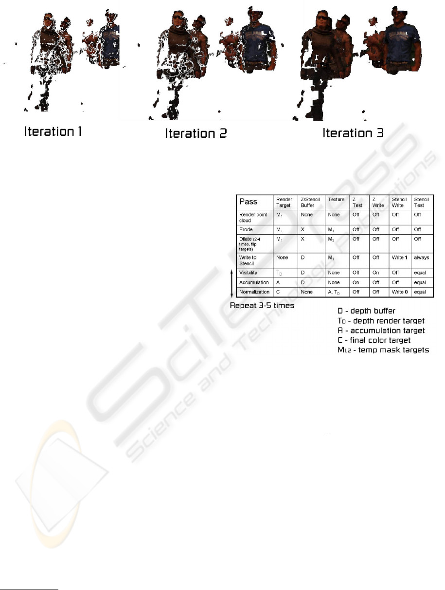
Figure 5: Adaptive Point Splatting performs multiple iterations over the point cloud. In each iteration, it relaxes the conditions

for pixel rejection.

der target while the other is set as a texture and vice

versa (Figure 6).

Once the mask texture is computed, a stencil

buffer of the original back buffer resolution needs to

be ﬁlled to be used by the iteration phase. To ﬁll the

stencil buffer, set the targets, disable color writing,

clear the stencil buffer, and render a quad that ﬁlls

the whole surface. Set the stencil buffer operation

to write the ﬁrst bit for every successful pixel. The

shader should read from the ﬁnal mask texture and

discard

pixels if the corresponding texture color is

zero. This will make sure only pixels that are set in

the original texture mask have their stencil bit set.

4.2 Executing an Iteration

During all 3 passes, the stencil buffer must be set to

only accept pixels whose corresponding stencil bit is

set. In the last normalization pass, the stencil buffer

also needs to reset the stencil bit of the accepted pix-

els so they aren’t modiﬁed in future iterations. The

ﬁrst two passes are generally the same as described

in (L. Ren and Zwicker, 2002) except that the ﬁrst

pass also renders the depth of each pixel to a sepa-

rate texture. This depth texture will then be used in

the normalization phase to ensure that accepted pixels

have the correct depth to be clipped properly by the

background geometry rendered up to this time. In the

second pass, we use the alpha channel to accumulate

the probabilities and the RGB channels to accumu-

late the color. One important implementation detail

when dealing with 16bit ﬂoating point render targets

is the precision. There are only 10 bits of precision,

so appropriate scaling in the probabilities is needed to

make sure ﬂoating point errors don’t occur.

In Cg, there is a discard command that implements this

behavior.

Figure 7: The render states for all the passes associated with

the Adaptive Point Splatting algorithm. Any number of it-

erations can be performed with 6 separate render targets;

therefore the memory complexity is constant with respect

to the iterations.

Altogether 3 ∗ num iterations + 6 passes are

needed for the whole algorithm.

5 EXPERIMENTAL RESULTS

All our experimental results were done on teleimmer-

sion data from UC Berkeley (of California Berkeley,

) where 48 cameras were capture the scene in real-

time. This data is then streamed to one computer act-

ing as the renderer. Besides missing information and

the typical rough estimates of the depths due to the

real-time stereo algorithm, camera calibration errors

persist. Sometimes three cameras could have face

information, but merging them won’t produce a co-

herent face because the three faces could be 1-2cm

GRAPP 2007 - International Conference on Computer Graphics Theory and Applications

232

off. The colors are also offset a little due to the dif-

fering lighting from each different location. In each

frame, the point clouds had roughly 75,000 points.

On a 2Ghz machine with a GeForce 6600 card render-

ing at 1024x768 resolution and performing three hole

ﬁlling passes and three iterations per frame, the algo-

rithm runs at 10.5 frames per second. Since the points

come from an image and a disparity map, we esti-

mate the normal of the surface of each point by ﬁtting

a plane to the neighboring points. We orient the quad

associated with each point to face the computed local

normal vector. Although computing the normals has

a small performance hit, we ﬁnd that the resulting im-

age quality is much better than with having the quads

always face the viewer. Figure 8 shows more compar-

isons of Adaptive Point Splatting and traditional point

cloud rendering.

6 CONCLUSION

We presented a GPU technique to deal with noisy

point clouds from stereo data. Such point clouds will

always be present since the stereo algorithms have to

run in real-time. The main incentive to use the GPU

for all processing is that the CPU is usually over-

loaded with many other tasks. Structuring the render-

ing algorithm such that no stalls occur between the

GPU and CPU means that the CPU doesn’t block on

any rendering calls and both processor can truly run

in parallel. Due to a GPU’s parallel processing na-

ture, GPU computing power seems to grow at a much

greater rate than CPU computing power; therefore,

GPU based algorithms will speed up at a greater rate

if their performance is GPU bound, which Adaptive

Point Splatting is. This type of ﬁltering is impossible

to do in real-time on today’s CPUs.

REFERENCES

Everitt, C. (May 2001). Interactive order-independent trans-

parency. In http://developer.nvidia.com/attach/6545.

H. Pﬁster, M. Zwicker, J. v. B. and Bross, M. (July 2000).

Surfels: Surface elements as rendering primitives. In

SIGGRAPH Proceedings.

Kalaiah, A. and Varshney, A. (June 2001). Differential point

rendering. In Proceedings of the 12th Eurographics

Workshop on Rendering.

L. Ren, H. P. and Zwicker, M. (2002). Object space ewa

surface splatting: A hardware accelerated approach to

high quality point rendering. In Eurographics.

Levoy, M., Pulli, K., Curless, B., Rusinkiewicz, S., Koller,

D., Pereira, L., Ginzton, M., Anderson, S., Davis,

J., Ginsberg, J., Shade, J., and Fulk, D. (July 2000).

The digital michelangelo project: 3d scanning of large

statues. In SIGGRAPH Proceedings.

Lien, J. and Bajcsy, R. (2006). Model driven compression of

3-d tele-immersion data. In Technical Report, EECS

Department, Universityi of California, Berkeley.

of California Berkeley, U. http://tele-immersion.citris-

us.org.

R Kolluri, J. S. and O’Brien, J. (2004). Spectral surface re-

construction from noisy point clouds. In Eurographics

Symposium on Geometry Processing.

R. Pajarola, M. Sainz, R. L. (June 2004). Extreme splatting:

External memory multiresolution point visualization.

In UCI-ICS Technical Report No. 04-14.

Remondino, F. (2006). Image-based modeling for object

and human reconstruction. In Ph.D Thesis ETH No

16562, Institute of Geodesy and Photogrammetry.

Stamminger, M. and Drettakis, G. (June 2001). Interactive

sampling and rendering for complex and procedural

geometry. In Proceedings of the 12th Eurographics

Workshop on Rendering.

REAL-TIME ADAPTIVE POINT SPLATTING FOR NOISY POINT CLOUDS

233

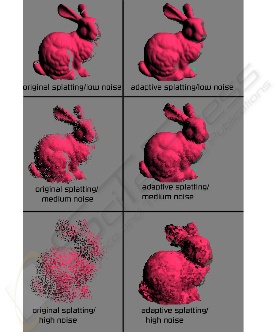
Figure 8: Example comparing the original splatting algorithm (left) with APS (right). Artiﬁcial noise was added to the point

clouds on the second and third rows in order to simulate similar irregularities as in the stereo data. Even with a lot of noise,

the APS rendering of the Stanford bunny looks solid and runs in real-time.

GRAPP 2007 - International Conference on Computer Graphics Theory and Applications

234