ON THE SEMI-AUTOMATIC VALIDATION AND
DECOMPOSITION OF TERNARY RELATIONSHIPS WITH
OPTIONAL ELEMENTS
Ignacio-J. Santos, Paloma Martínez Fernandez and Dolores Cuadra
Departamento de Informática de la Universidad Carlos III de Madrid Av. Universidad 30 – 28911 Leganés (Madrid)
Keywords: Cardinality Constraint, Entity-Relationship Model, Relational Model, Semantic and Syntactic Anomalies,
CASE (Computer Aided Software/ Engineering) Tools.
Abstract: This paper analyzes the problems that concern the design of databases. CASE tools supply a resources kit
for the design and creation of database in a DBMS (Database Management System). Sometimes, these tools
only help to draw diagrams. Ideally, they would verify and validate DB design and transform it from
Conceptual to Logical Model. In a last step, they would transform the Logical Model to a specific DBMS.
Currently, commercial tools do not verify or validate the model in an optimal way. This paper is focused on
the validation and checking of database schemas. This work specially analyzes the ternary or higher-order
relationships when there are optional components.
1 INTRODUCTION
When a Project Leader develops an application from
the beginning, he or she has to think in the data.
Once the designer has created the Conceptual
Schema, the designer has to transform the
Conceptual to Logic schemas, because the Logic
Model is nearest to a DBMS. This paper is focused
on Entity-Relationship and Relational models. A
CASE tool of Database helps to realize the scheme
in a particular DBMS. These tools start helping to
design the Conceptual Model from UD and after
they transform this Conceptual to Logic Model. At
the end, they create a schema in a SGBD.
A scheme has to be verified syntactically and
semantically. The syntactical verification has to
check the rules of building. The semantic
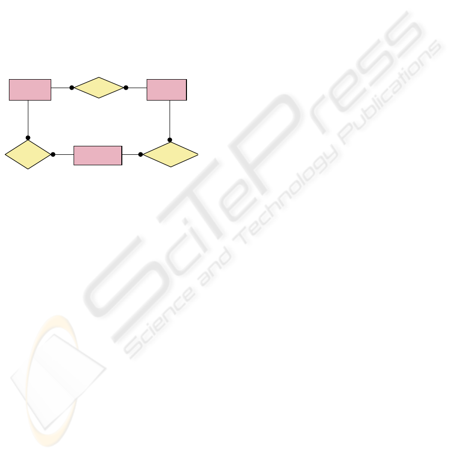
Fi
g
ure 1: Valida
t
ion and Verification of a Schema.
465
Santos I., Martínez Fernandez P. and Cuadra D. (2007).
ON THE SEMI-AUTOMATIC VALIDATION AND DECOMPOSITION OF TERNARY RELATIONSHIPS WITH OPTIONAL ELEMENTS.
In Proceedings of the Ninth International Conference on Enterprise Information Systems - DISI, pages 465-472
DOI: 10.5220/0002386804650472
Copyright
c
SciTePress

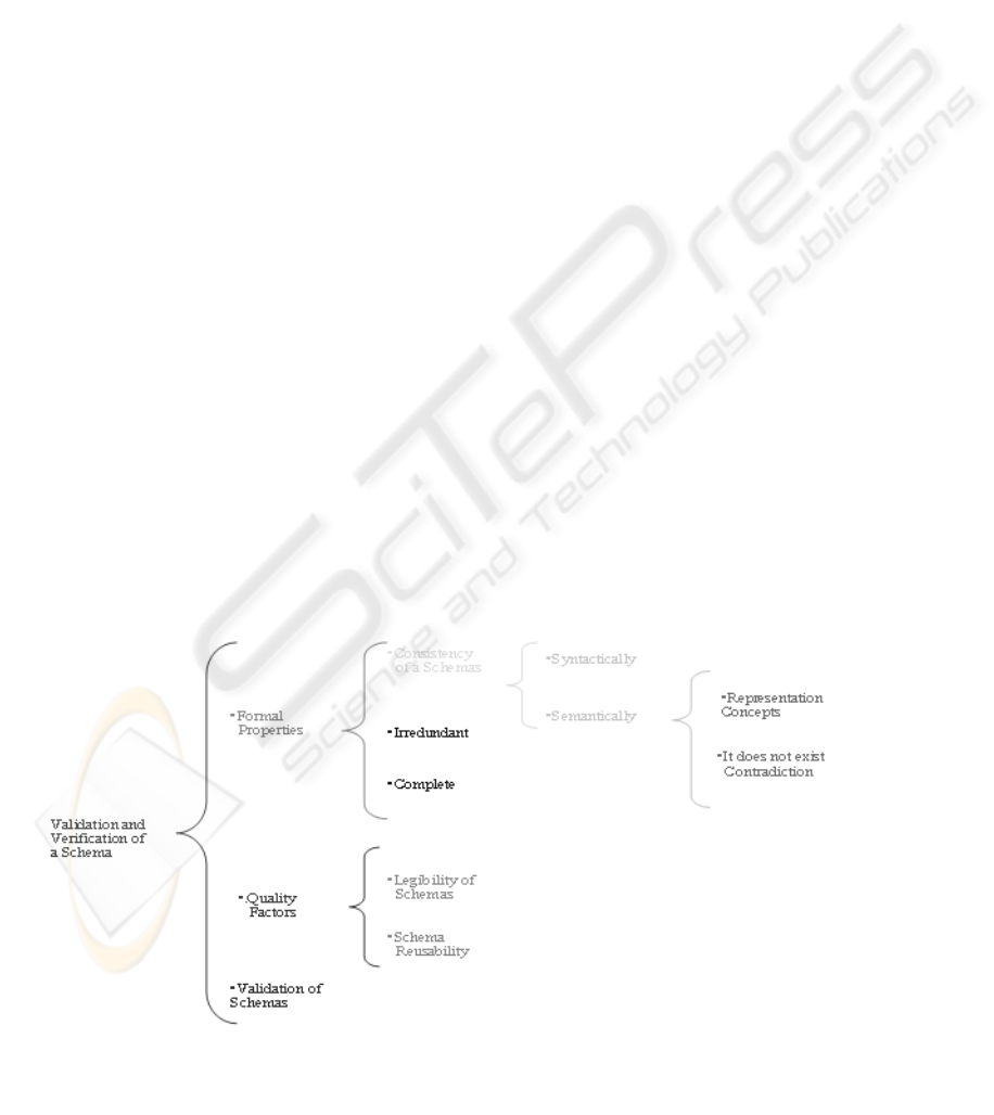
verification tries to find the inconsistency between
the semantic constrains and the user (Bouzeghoub,
M. et al., 2000). The figure 1 shows the steps of
validation and verification of a scheme. A good
Conceptual scheme has to have Formal Properties,
Quality Factors and Conformance with the user
necessities (validation). Formal properties mean that
the scheme has to be consistent, complete and
irredundant. With respect to formal properties the
majority of commercial CASE tools do a good
syntactic validation, but no semantic. For example,
they check if there is, at least, an entity and that the
entities have different names. However, they do not
check if there are contradictions among the schema
concepts. These tools do not also verify the
redundant elements. The completeness of a
Conceptual scheme can be defined with respect to
the meta-model or the UD represented. The first part
the metamodel concerns the mandatory elements
that constitute a conceptual schema. The commercial
tools do this verification. The represented UD means
the validation with respect to the user requirements.
Checking whether a Conceptual schema represents
all the necessary knowledge for a given information
system, which refers to conformance of the
Conceptual schema to the real world. With respect to
quality factors, we have to look at the things the
readability and the reusability. Readability is a
desirable property, but it is a subjective valuation.
The reusability is far away in commercial tools. For
the last, the validation of a schema means that if the
schema is adapted to the user requirements. In this
topic, some tools have developed the Paraphrasing
(NLDB, 2000). This technique generates a textual
description from a Conceptual schema and the user
can validate the model.
This paper analyzes the validation and
correctness of the ternary or higher order
relationships with optional elements. The majority of
tools do not well implement this type of
relationships.
Next section will describe the necessary
definitions for this paper. The third section will look
over some research works about this topic. The
fourth section will explain our contribution and it
will analyze and validate the relationships with
optionality. The fifth section will observe the
semantic anomalies in the ternary relationships with
optional elements. The sixth section will show with
an example our proposal. The seventh section will
show the conclusions.
2 SOME REQUIRED
DEFINITIONS
We show in this section the necessary definitions for
developing this paper. We begin by defining the
Entity and the Relationship element according to
Thalheim (2000).
Let be
(
)
{
}
(
)
njid
jn
≤≤Ε
Α
Α
=
Ε
1/,...,
1
an entity
with attributes
n
Α
Α
,...,
1
, each attribute is defined in
a domain, where
(
)
{
}
njid
j
≤≤
Ε
1/
is the set of
candidate keys of the entity E, and this property
characterizes in a univocal way, every one of the
instances of E. We define
t
E
as a set of instances of
E. An element
t
e
of
t
E
is a vector of n values, where
the component i is denoted by
()
ii
dome Α∈
, which
verifies that everywhere instance
t
e
'
and
(
)
Ε
j
id
:
()
(
)
≠Π
Ε
t
id
e
j
()
(
)
t
id
e
j
'
Ε
Π
where
()
ΕΠ
Α
is the
projection of A in E.
We define the set of key instances associated to
an entity as
(
)
t
Ε=Ε
ΙΡ
π
#
. A relationship of order n
with s attributes is defined as
R=
(
)
sjn
r ΑΑΕΕ ,...,,,...,r
111
, where each
i
r
is the role
and, where the entity
Κ
Ε
participates in R. We
define
t
R
as the set of instances of R. An
element
t
r
of this set is a vector of n components,
where each component depicts a role that contains a
key instance of the entity that it takes part with this
role. Then, the set of instances
t
R
of a relationship R
is a subset of the product contained of the key
instances of the entities that participate in R and
domains of attributes that participate in R.
() ()
sjn
t
domdomErErR Α××Α×××⊆ ......
111
.
We define the participation cardinality
constraint of an entity
(
)
RrC
ji
,Ε
= {0 or 1} as the
optional or mandatory participation, respectively, of
the key instances
j
E
with role
j
r
in the relationship
(
)
jn
rrR ΕΕ= ,...,
11
where the relationship has order n.
Optional constraint is depicted with a white circle,
and the mandatory with a black circle, but both by
the side of the relationship.
The Merise’s cardinality for a relationship is
defined as CMerise
),( REr
ji
= (n, m) where
i
r
is the
role in
(
)
jn
rrR ΕΕ= ,...,
11
,
mn
≤
, and n, m
Ν
∈
. This
means that a key instance of
t
ji
REr ∈
is in
t
R
as
minimum and maximum n, m times. We depict this
cardinality with a label at the end of the line that
ICEIS 2007 - International Conference on Enterprise Information Systems
466

links the entity and the relationship but by the side
of the relationship.
The Chen’s cardinality (Cuadra, 2003) for a
role
i
r
into
(
)
jn
rrR ΕΕ= ,...,
11
as CChen
(
)
Rr
ji
,Ε
= (n, m),
where n, m
Ν
∈ and
mn
≤
≤1
. This means that for
any combinations of key instances
t
nii
Rdeaaaa ,...,,,...,
111 +−
is in
t
R
, n and m times as
minimum and maximum, respectively. We depict
this cardinality in a label at the line that links the
entity and the relationship but by the side of the
entity.
Let be R=
(
)
jn
ErEr ,...,
11
a relationship of grade
n. We define a Complementary Relationship of R
(Cuadra, 2003) as
c
a
R
, where a shows the roles in
which participates this relationship and it has to
carry out:
a<n, that is to say, the number of roles which
are applied, it has to be less than the grade of
the relationship.
Let C(aE, R)=0 be the cardinality constraint
for every entity, which participates with every
one of the roles in E has to be optional.
RR
c
a
⊄
, that is to say, the instances which
belong to the relationship, they can not be a
subset of the complete relationship.
Let be R=
(
)
jn
ErEr ,...,
11
a relationship of order
n. We define a Complete Relationship of R as
T
a
R
,
with the same definition of the Complementary but
it does not carry out the third point.
We use some definitions from the work of
Trevor H. Jones and Il Yeol Song (Trevor H. Jones
et al., 1996). If a binary relationship is semantically
a subset of the ternary relationship and constraints
the instances of the ternary relationship, then the
binary relationship is a Semantically Constraining
Binary (SBC) relationship. If not the binary
relationships is Semantically Unrelated Binary
(SUB) relationship. We do not analyze the SUB
because it has not an effect on the ternary. They
define the Implicit Binary Cardinality (IBC) rule as
in any given ternary relationship, regardless of
ternary cardinality, the implicit cardinalities between
any two entities must be considered M:N, provided
that there are no explicit restrictions on the number
of instances than can occur. They define the Explicit
Binary Permission (EBP) rule for any given ternary
relationship, a binary relationship cannot be imposed
where the binary cardinality is less than the
cardinality specified by the ternary, for any specific
entity. In addition, the Implicit Binary Override
(IBO) rule is given the imposition of a permitted
binary relationship on a ternary relationship, the
cardinality of the binary relationship determines the
final binary cardinality between the two entities
involved.
McAllister, A. (1997 and 1998) defines the
MX2 rule, denoted as augmentation rule. He defines
r as the total set of roles for a relationship R. The
cardinality constraint Cmax(a, b) means that if we
fix a role [a] is the number maximum [a, b]
permitted in R. The augmentation rule (MX2)
defines that Cmax (a, b)
≤
Cmax (ac, b). The MX2
rule is equivalent to the Explicit Binary Permission
(EBP) rule.
On the other hand, we use some definitions of
the Relational Model. They are definitions of Millist,
W. V. (1994). Let t be a tuple of a relation R. Let
*
t
be a tuple to insert, update or delete. Let
Κ
∑
be the
set of key dependencies. The set of all relations that
they satisfy
Κ
∑
is denoted as SAT (
Κ
∑
).
Let R be a relation,
∑
a set of dependencies,
which apply to R and, r(R) a relation. A tuple
*
t
is
said to be compatible with r if
}{
*
tr ∪
is a relation
which is in SAT (
Κ
∑
).
3 RESEARCH ABOUT THE
VALIDATION OF TERNARY
RELATIONSHIPS
In this section, we analyze different proposals about
the validation and verification of relationships.
Trevor H J., et al. (1996) focus on cardinality
constraints associated to ternary relationships. They
analyze the SBC relationships and as they can affect
to cardinality constraints in the ternary relationship.
They analyze the implicit and explicit binary
relationships and demonstrate their theories through
the functional dependencies. The proposal does not
depict the syntactic or semantic anomalies, they only
study the semantic associated to ternary relationship
through binary relationships. The paper of James
Dullea (Dullea, J. et al., 1998) depicts when an E/R
diagram has not redundancy. They do an analysis
about the path (cycle path), which can be right or
wrong. They analyze the optionality and they study
its cardinality. However, they do not look at the E/R
model anomalies.
The papers of McAllister, A. (1997 and 1998)
describe an analysis about the minimum and
maximum cardinality constraints in the
relationships. He establishes rules for deducing
cardinalities in the schema. If we apply these rules is
ON THE SEMI-AUTOMATIC VALIDATION AND DECOMPOSITION OF TERNARY RELATIONSHIPS WITH
OPTIONAL ELEMENTS
467

possible to get a simplification or decomposition of
the original schema. However, these works do not
explain the problem from the UD. His work shows
the minimum cardinality, 0, but he does not resolve
the semantic problem of the optionality.
Rafael Camps (Camps, R. 2002) depicts an
excellent analysis about the transformation of
ternary relationships, with and without imposition
binaries from E/R to R Model. In his work he
establishes that the “Look across” cardinality
constrains with the Chen approximation is richer
semantically. We think also it. Furthermore, he
shows the problem that the transformation from E/R
to R using only functional dependencies has
semantic anomalies.
In the R Model Millest W. Vicent (Millist W.
Vincent, 1993, 1994, 1999) describes the semantic
anomalies that have the relationships.
Santos (Santos, I. et al., 2006) depicts the semi-
automatic validation and decomposition of ternary
relationships, however this work does not analyze
the optionality.
4 VERIFICATION AND
VALIDATION OF TERNARY
RELATIONSHIPS WITH
OPTIONALITY
We use the representation of “Look across”
cardinality constraints of Chen and Merise
approximations (Cuadra, 2003), because the
depicted semantic is very good for the automation in
a CASE tool. The Chen approximation can be use
for deriving the functional dependencies. We use the
MX2 rule of McAllister for validating the
Conceptual schema. On the other hand, the “Look
across” cardinality constraint with Merise
approximation shows us the primary key and, the
candidate keys, if they exist. Furthermore, with this
approximation we can get complex rules, because
the value of an attribute in a relationship for a
domain as minimum has to be n and as maximum m
times,
Ν
∈∀ mn,
(Al-Jumaily, T. H., 2006).
When there are optional elements in a ternary
relationship, we have problems in its transformation.
A solution is the Complementary binary relationship
(Cuadra, D., 2003). In this work, we propose also
the Complete binary relationship. Both solutions
were defined in the second section. The
Complementary relationship is a good solution,
because it has not redundancy. However, in the
Complete, there is redundancy, but it will be good
solution when there is decomposition.
Next, we show two algorithms of validation and
simplification of ternary relationships. Theses
algorithms are a modification of Santos, I, (Santos, I.
et al., 2006). We begin by checking the schema
semantic consistency. In a next step, we have to
verify if the concepts are according to the definition
and, there are not incompatibilities among the
concepts and the schema.
In this paper, we analyze only the ternary or
higher-grade relationship. For this when we find a
ternary relationship in our model,
i
R
, we have to
look for the SBC relationship with
i
R
. For each
entity
i
Α
related to
i
R
, we have to find other
relationships
j
R
, with
ji
RR
≠
, and the rest of entities
{
}
nii
Α
Α
Α
Α
+−
,...,,,...,
111
which are related to
i
R
.
These relationships that we find, they are candidates
to be semantic related relationship to
i
R
, and for this,
they can restrict the cardinality of the
relationship
i
R
. When we have the relationships, we
have to ask to the designer, because he/she has to
decide the relationships, which are SBC.
The step next is to check the optional roles of
the entities in the ternary relationship. Let be
i
Ε
,
j
Ε
and
Κ
Ε
∈
i
R
. If
i
Ε
has an optional role, then we
build between
i
Ε
and
j
Ε
the Complementary binary
relationship. However, if between
i
Ε
and
j
Ε
there is
an implicit ternary relationship, then we can build
the Complete binary relationship and we delete the
implicit binary relationship.
Now we show the algorithm of validation of a
relationship with optionality.
The first algorithm depicted in the figure two
has the follow steps:
1. We get the ternary relationship and SBC
relationships with the ternary to check,
with the help of the designer.
2. Are there some optional elements in the
ternary relationship?
3. If there are optional roles then we build
the Complementary or Complete binary
relationships.
4. We verify the Conceptual Design with
the MX2 rule of McAllister. Do the
relationships carry out MX2? We have
to verify the rule
(
)
2/123
1
+−
−nn
times.
ICEIS 2007 - International Conference on Enterprise Information Systems
468
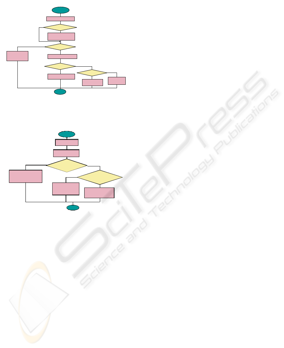
Figure 2 : Validation of Relationship with optionality.
Figure 3.- SIMPL IF ICATION ALGORITHM O F A RELATIONSHIP
Begin
1. -W e get the r el ati onship
Of t he al gorit hm one.
2 .-S ynthesi s or A nal ys i s
al gorithm
3.- Is i t in BC NF? And Has not
Information l osses and preserv e
F uncti onal d ependenci es?
End
4. - Decom position wit h semantic
anomal ies
-
6. - T he decompo si ti on has
I nforma tion is lo ss es
7. - The de com po si tion is we ll,
wit hout s emantic ano ma lies.
No
Yes
5. - bel o ng s to
Relationships of the
dec o mp osi t io n?
No
Ye s
C
RorR
Τ
Figure 3 : Simplification Algorithm of a Relationship.
5. Design is incorrect. The E/R Model has
to be redesigned.
6. We transform the design from E/R to R
Model getting the functional
dependencies. We can get the FD from
“Look Across” cardinality constrains
with the approximation of Chen. We
have a FD if maximum cardinality is
one. After, with the classic algorithms
we verify the normal form of the
schema.
7. Is the schema in the Boyce Codd
Normal Form?
8. If the schema is in BCNF, the design is
good and it has not semantic anomalies.
9. Is it in 3NF?
10. Design good, but with semantic
anomalies. We could use the second
algorithm.
11. Design with semantic anomalies. We
ought to use the second algorithm.
If a ternary relationship with optionality can be
decompose and the decomposition or simplification
is in BCNF, this decomposition will always have
information losses if the Complementary (
C
i
R
) or
the Complete (
T
i
R
) relationship are not in the
decomposition.
Theorem: Let be relation schema R and let be
Τ
R
a Complete binary relationship and let be
C
R
the
Complementary.
The decomposition is in BCNF.
Let
n
RRR ,...,,
21
be a set of relationships of the
decomposition of R. The
n
RRR ,...,,
21
R∈ is
information lossless and functional lossless.
If
T
R
or
i
C
RR ≠
, where
Ni ∈
, then the
decomposition is information loss.
Proof: If
T
R
or
i
C
RR ≠
will not be the original
tuples, because
n
RRRR ><><>< ,...,
21
=
.
The algorithm implemented in the figure three
shows the steps of simplification of a ternary
relationship with or without optional elements.
1. We get the relations from algorithm
first.
2. We apply the Analysis or Synthesis
classic algorithms.
3. Is the result in BCNF? Does not it
exists information losses and preserve
functional dependencies?
4. The decomposition has semantic
anomalies. It is not good solution.
5. Are there Complete relationships?
These relationships belong to
decomposition?
6. The decomposition has information
losses.
7. The decomposition is valid.
We prefer the Complete relationship to the
Complementary, only in this case, because if we use
Complementary then we have to do an union
between the Complementary and its
corresponding
i
R
.
Fi gure 2.- VAL IDATI ON OF A R EL ATI ONSHI P W HITH OPTI ONALI TY
Begi n
1.-We get the rel ationships
2.-Are there optional
elements?
3.-We c reat e Co m pl eme n ta r y
or Complete relationship.
4.- MX2?
6.-We get the Normal From.
7.- Is i t i n BCNF?
8.-The design is val id.
End
5.-The relationship is not
val i dat e d
9. Is it 3 NF?
10.-Design val i d but
Semanti c anomal ies
11.- Desig n is not
val i d
No
Yes
Yes
No
Yes
No
No
ON THE SEMI-AUTOMATIC VALIDATION AND DECOMPOSITION OF TERNARY RELATIONSHIPS WITH
OPTIONAL ELEMENTS
469
5 ANOMALIES IN THE
COMPLEMENTARY
RELATIONSHIPS
When there is a ternary relationship, with or without
imposition binaries but with at least a
Complementary binary relationship, the insertion,
deletion, updated and selection operations have
anomalies. We will analyze in this section these
problems. For this analysis we have use the
definitions of Millis W. Vincent (Millist W. Vincent,
1993, 1994, 1999).
Let be three entities E, P and T, a relationship R
with attributes e, p, t and a Complementary
relationship ought to T is optional. In the insertion,
we will have to distinguish when we insert a null or
not.
1. Let
*
t
=<e,p,null> be a tuple to insert
and let r(R) the ternary relationship
and let
(
)
cc
Rr
be the Complementary
relationship. If
{
}
(
)
(
)
Κ
Σ∈∪ SATtr
*
and
{
}
(
)
()
Κ
Σ∈∪ SATtr
c *
then we
can insert
>=< pet
c
,
*
in
c
R
.
2. Let be t=<e,p,t>,
nullt ≠
and let r(R)
be the ternary relationship and
(
)
cc
Rr
the Complementary. If
{
}
(
)
∈∪
*
tr
()
Κ
ΣSAT
and
{
}
(
)
∈∪
*
c
c
tr
(
)
Κ
Σ
SAT
,
then we can insert
*
t
in R.
The delete operations have two cases.
1. Let
*
t
=<e,p,t>, where t=null. If
{
}
(
)
(
)
Κ
Σ∈− SATtr
c
c *
, then we can delete
*
c
t
in
(
)
cc
Rr
.
2. Let
*
t
=<e,p,t>, where
nullt ≠
. If
{
}
(
)
(
)
Κ
Σ∈− SATtr
*
, then we can
delete
*
t
of R.
However, the modification operations have four
cases.
1. Let be t=<e,p,t> and
*
t
=<e’, p’, t’>,
where t, t’
null≠
. If
{
}
(
)
(
)
∈−∪ trt
*
(
)
Κ
ΣSAT
, then the modification is
right and we update only the ternary.
2. Let be t=<e,p,t> and
*
t
=<e’, p’, t’>,
where t and t’= null. If
−∪
c
c
rt (}({
*
))
*
c
t
()
Κ
Σ
∈ SAT
then the modification
is possible, but in the Complementary.
3. Let be t=<e,p,t> and
*
t
=<e’,p’,t’>,
where t=null and t’
null≠
. If
{
}
(
)
()
Κ
Σ∈− SATtr
c
c *
and
{
}
(
)
∈∪
*
tr
(
)
Κ
Σ
SAT
, then we can delete
c
t
of the
Complementary and to insert
*
t
in the
ternary.
4. Let be t=<e,p,t> and
*
t
=<e’,p’,t’>,
where t
null
≠
and t’=null. If
{
}
(
)
()
Κ
Σ∈− SATtr
*
and
{
}
(
)
∈∪
*
c
c
tr
(
)
Κ
Σ
SAT
, then we can delete t of
ternary and to insert
*
c
t
in the
Complementary.
The operation of selection is more complex:
Select e, p, t from ternary-relationship
Union
Select e, p, null from Complementary;
When there is decomposition and a binary
relationship is overlapped by the Complementary
relationship is better to replace the relationships by
the Complete relationship.
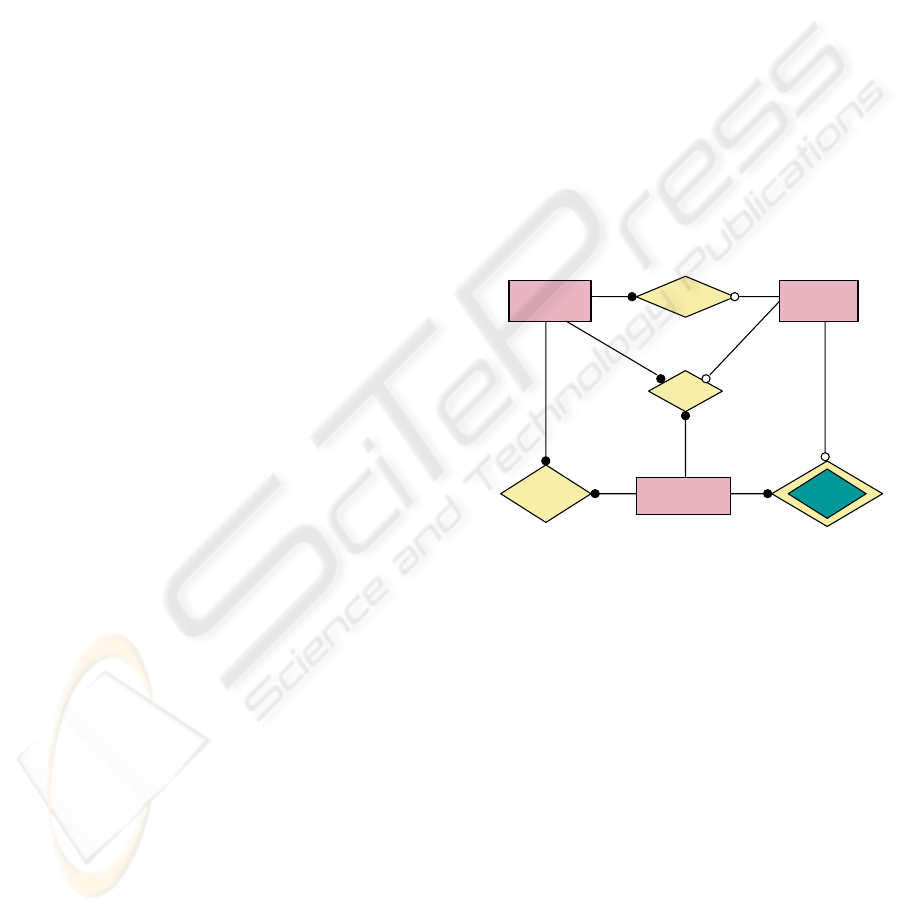
Figure 4 : Case (i).
6 VALIDATION AND REFINING
OF TERNARY RELATIONSHIP
AND ITS DECOMPOSITION
WITH OPTIONALITY
Let be a company that wants to manger the jobs and
employees. The management has imposed the next
constraints:
• An employee that works in a project, he can
only use a technique.
• An employee that works at a technique, he
can only work at a project.
• An employee can only work at a unique
project.
Figure 4, . Case (i)
-
Tec hni q ue
Pr oj ec t
Pr oj ec t-
Tec hni q ue
Job
Empl o yee-
-Project
Empl o ye e
Empl o yee-
- Tec hni q ue
(1,1)
(1,1)
(1,1)
(1,1) (1,1)
(1,1)
(1,1)
(1,1)
(1,n
(1,n)
(0,n)(1,n)
(0,n)
(1,n)
(0,n)
(1,1)
(0,n)
(1,n)
ICEIS 2007 - International Conference on Enterprise Information Systems
470
• In a project is only possible use a
technique.
• The last constraint, we distribute in two
exclusive cases in our example:
(i) It can have employees with projects
that they do not have allocated
technique.
(ii) It can have employees that use a
technique, but they are not allocated to
any project.
Figure 5,. Case ( ii)
-
Te c h n iq u e
Pr oj ec t
Project-
Technique
Job
Employee-
-Project
Employee
Employee-
-Technique
(0,n)
(0,1)
(1,1)
(1,1)
(1,1)
(1,1)
(1,n)
(1,1)
(1,1)
(0,n)
(1,n)
(1,n)(0,n)
(1,n)
(1,n)
(1,n)
(1,n)
(0,n)
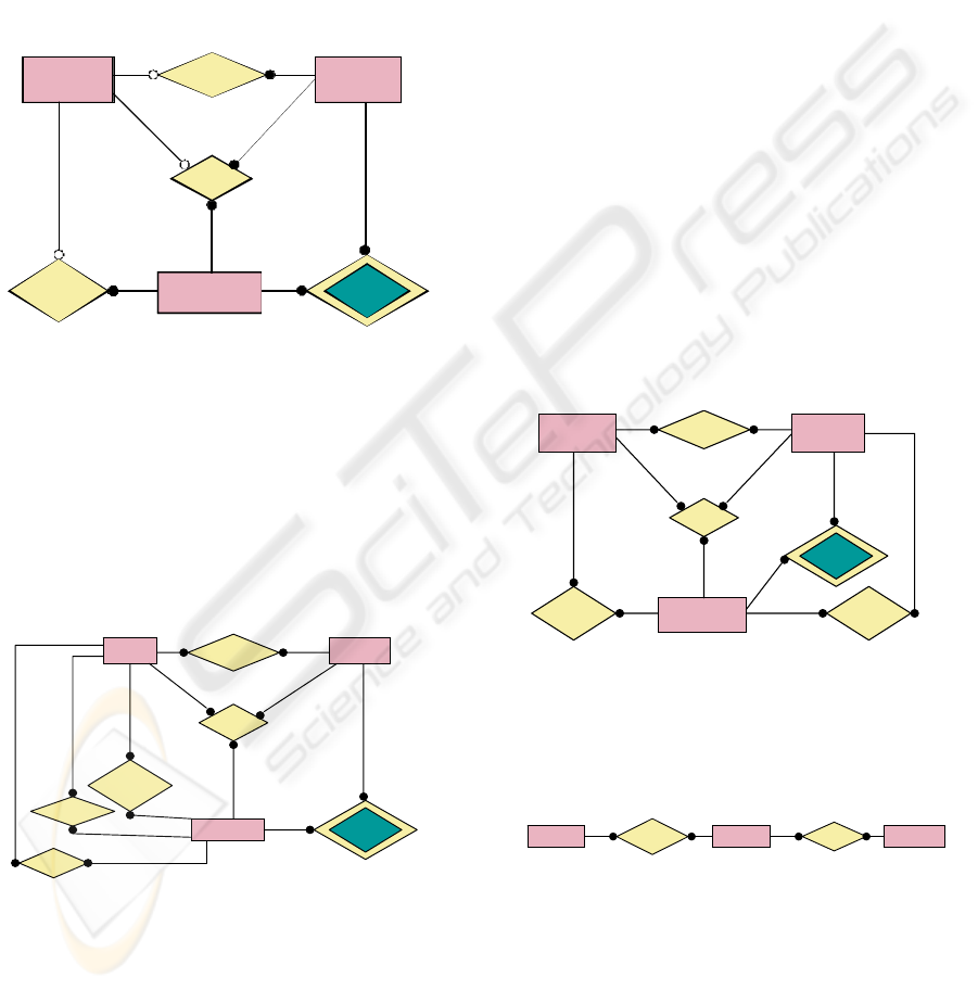
Figure 5 : Case (ii).
We show in the figure fourth and fifth the E/R
model of this example. In the figure sixth (case (i))
and seventh (case (ii)) is the solution to optional
elements, with the Complementary binary
relationship. From the figure forth, we depicts the
“Employee-Technique” relationship with double
rhombus, because it is a deduced relationship.
Figure 6 : We transform the optionally case (i).
Through the algorithm one, we verify the
relationships and we look at the redundancies.
We can notice that in both cases that carry out
the augmentation rule (MX2 rule).
If we get the functional dependencies, in both
cases we have:
Σ
= {(Employee, Project
→
Technique; (Employee, Technique)
→
Project;
Employee
→
Project; Project
→
Technique}. The
Key is
Κ
S
={Employee} and the minimum cover
m
R
= {Employee
→
Project, Project
→
Technique}. The
resulting schema is in the 2NF.
If we apply the second algorithm, then we will
get two relations;
1
R
={Employee, Project} with
1
Σ
= {Employee
→
Project} and
2
R
={Project,
Technique} with
2
Σ
={Project
→
Technique}.
If we go on the case (i), we replace
1
R
={Employee, Project} and the Complementary
relationship by the Complete relationship. In the
figure eight depicts this case.
However, in the case (ii), this is not right,
because, we lose data. The Complementary is not in
the decomposed relationships. Furthermore, we can
not select
1
R
={Employee, Project} with
1
Σ
=
{Employee
→
Project} and
3
R
= { Employee,
Technique} with
3
Σ
= { Employee
→
Technique}
because we have dependency loss in this
decomposition. Then, the decomposition is not valid,
as we depict in the figure nine.
Figure 7 : We transform the optionally Case(ii).
We can resume that the decomposition or
simplification of the relationships, although this is in
Figure 8 : Simplification of Case (i).
FNBC, if in the decomposition are not
complementary relationship, the decomposition is
not valid.
Fi gure 6,. We transfor m the optional l y case (i)
-
Tec hni q ue
Pr oj ect
Pr oj ect -
- Tec hni q ue
Job
Empl oyee
Empl oyee-
- Tec hni q ue
(1,1)
(1,1)
(1,1)
(1,1)
(1,1)
(1,1)
(1,1)
(1,1)
(1,1)
(1,n)
(1,n)
(0,n)
(1,n)
(1,n)
(1,n)
(1,n)
(1,1)
(1,n)
Emp l o yee-
-Project
Compl em ent ar y
Comple te
(1,n)
(1,1)
(1,1)
(1,1)
(1,n)
(1,n)
(1,n)
(1,n)
Figur e7, . We trans for m the o pti onal l y of Case (i i )
-
Tec hniqueProject
Project-
Technique
Job
Employee-
-Project
Employee
Employee-
-Tec hnique
(1,1)
(1,1)
(1,1)
(1,1)
(1,1)
(1,1)
(1,1)
(1,1)
(1,1)
(1,n)
(1,n)
(1,n)(1,n)
(1,n)
(1,n)
(1,n)(1,n)
(1,n)
Compl ementary
(1,n)
(1,n)
(1,1)
(1,1)
Figure 8, . Simplification of l Case (i)
Empl oyee
Pr oj ect
(1,1)
(1,1)
(1,1)
(1,n)
(1,1)
(1,n)
(1,n)
(1,n)
Compl et e
Pr oj ect -
Tec hni q ue
Tec hni q ue
ON THE SEMI-AUTOMATIC VALIDATION AND DECOMPOSITION OF TERNARY RELATIONSHIPS WITH
OPTIONAL ELEMENTS
471
7 SOME CONCLUSIONS
The design of a Database is a complex work. The
CASE tools help to simplify validation, verification
and simplification of a Database design. However,
these tools do not implement theses properties or
they are very far away.
This paper is based on the ternary relationships,
but it ought to be extended to higher grade ones.
Two algorithms for verifying, validating and
decomposing relationships with or without optional
elements have been shown. However, this work is
limited to functional dependencies and not to
multivalued (MVDs) or join (JDs) dependencies. On
Figure 9 : We transform the optionally case(i).
the other hand, we can conclude that sometimes
the simplification is not the better solution, because
of the anomalies.
REFERENCES
Bouzeghoub, M., Kedad, Z., Métais, E. “CASE Tools:
Computer Support for Conceptual Modeling”, chapter
13 of “Advanced Database Technology and Design”
of Piattini, M. and Díaz Oscar. Ed. Artech House, Inc.
2000.
Camps, R. (2002) “From Ternary Relationship to
relational tables: A case against common beliefs”.
ACM/SIGMON Record 31, July 2
nd
2002.
Cuadra, D. (2003). “Aproximación formal a las
restricciones de cardinalidad en un marco
metodológico de desarrollo de Bases de Datos”.
Doctoral thesis. Carlos III University of Madrid.
Computer Science Department.
Dullea, James and Il Yeol Sung (1998). “An Analysis of
the Structural Validity of Ternary Relationships in
Entity Relationship Modeling”. CIKM, pages 331-
339.
Al-Jumaily, Harith T. (September 2006). “Aplicación de
Técnicas Activas para el Control de Restricciones en
el Desarrollo de Bases de Datos”. Doctoral thesis,
Carlos III University of Madrid, Computer Science
Department.
McAllister, Andrew. (1997). “ Complete roles for n-ary
relationship cardinality constraint”. Data &
Knowledge Engineering 27 pages 255-288.
McAllister Andrew J. and Sharpe David. February 1998.
“An approach for decomposing N-ary Data
Relationships”. Software-Practice &Experience 28(2),
pages 125-154.
Millist W. Vincent and Bala Srinivasan. (1993). “A Note
on Relation Schemes which are in 3NF but not in
BCNF”, in Information Processing Letters 48 page
281-283.
Millist W. Vincent. 1994. PH. D. Thesis, “Semantic
Justification for Normal Forms in Relation Database
Design”, Department of Computer Science, Monasch
University.
Millist W. Vincent. (1999). “Semantic Foundations of
4NF in Relational Database Design”. In Acta
Informática 36, pages 173-213.
NLDB’2000 5th International conference on Applications
of Natural Language to Information Systems.
Versailles (France), June 28-30, 2000.
Santos, I., Martinez Fernández, P. and Cuadra Fernández,
D. (25-28 February 2006). “On the Semi-Automatic
Validation and Decomposition of Ternary
Relationships”. IADIS, 2006.
Thalheim, Bernhard 2000. “Entity-relationship modeling:
foundations of database technology”. Publishing:
Springer.
Trevor H Jones and Il-Yeol Song. (1996), “Analysis of
Binary/Ternary Cardinality Combinations in Entity-
Relationship Modelling”. Data & Knowledge
Engineering, Vol. 19, n 1 pages 39-64.
Figure 9, . Decomposit ion Case ( ii)
-
Tec hni q ue
Pr oj ect
Pr oj ect -
Tec hni q ue
Pr oyec t-
Empl o yee
Empl o yee
(1,1)
(1,1)
(1,1) (1,1)
(1,1)
(1,1)
(1,n)
(1,n)
(1,n)
(1,n)
(1,n)
(1,n)
Compl ement ar y
ICEIS 2007 - International Conference on Enterprise Information Systems
472
