BACKGROUND SEGMENTATION IN MICROSCOPY IMAGES

. J. Charles, L. I. Kuncheva

School of Computer Science, University of Wales, Bangor, LL57 1UT, United Kingdom

B. Wells

Conwy Valley Systems Ltd, United Kingdom

I. S. Lim

School of Computer Science, University of Wales, Bangor, LL57 1UT, United Kingdom

Keywords:

Image processing, image analysis, segmentation, background removal, microscope, vignetting, microfossils,

kerogen, palynofacies, palynomorphs.

Abstract:

In many applications it is necessary to segment the foreground of an image from the background. However

images from microscope slides illuminated using transmitted light have uneven background light levels. The

non-uniform illumination makes segmentation difﬁcult. We propose to ﬁt a set of parabolas in order to segment

the image into background and foreground. Parabolas are ﬁtted separately on horizontal and vertical stripes of

the grey level intensity image. A pixel is labelled as background or foreground based on the two correspond-

ing parabolas. The proposed method outperforms the following four standard segmentation techniques, (1)

thresholding determined manually or by ﬁtting a mixture of Gaussians, (2) clustering in the RGB space, (3)

ﬁtting a two-argument quadratic function on the whole image and (4) using the morphological closure method.

1 INTRODUCTION

Images with non-uniform background illumination

appear in various applications, e.g., in biology,

medicine, astronomy and geology. Most cases of un-

even illumination occur when taking images through

a microscope or telescope. The periphery of the im-

age is usually poorly illuminated and this is known as

vignetting. There are three main types of vignetting,

mechanical, optical and pixel. Mechanical vignetting

is caused by the physical construction of the optical

viewing device while optical vignetting is inherent in

the lens design. Pixel vignetting only occurs in digi-

tal cameras due to less light hitting a photon cell at an

oblique angle, i.e., towards the edges of the image.

The microscopy images of interest in this study

come from rock and drill cuttings and contain mi-

crofossils and other organic debris on a light back-

ground. The images are taken with transmitted light

microscopy. The concentrated light source com-

pounds the effect of vignetting causing even worse il-

lumination across the image. The background is typ-

ically brighter in the middle and darker towards the

edges.

The most common method to segment the fore-

ground from the background of an image is thresh-

olding (Otsu, 1979; Cinque et al., 2004; Sankur and

Sezigin, 2004). However, using a constant thresh-

old will result in objects of interest near the edges of

the image being lost within a “rim” labelled as fore-

ground. On the other hand, light objects in the middle

of the image will be blended with the background. In

this case global thresholding will have to be replaced

with local thresholding. To perform local threshold-

ing a background estimate is required so that an in-

dividual threshold is set for each pixel. A common

method for obtaining this estimate is to use the image

of an empty microscope slide as a template. However

a single estimate may not be suitable for all images

due to possible changes in the microscope setup. This

is why we seek a method for unique background es-

timation based solely on the image provided. It has

been shown that as the light intensity fades with the

square of the distance from the source, a quadratic

function can be used to model the illumination (Mon-

tage, 2002). Higher order surface polynomials have

also been used but, typically these are applied to im-

ages captured using techniques where vignetting is

not the cause of uneven illumination (Zawada, 2003).

These single-function models may be too coarse and

139

Charles J., Kuncheva L. and Wells B. (2008).

BACKGROUND SEGMENTATION IN MICROSCOPY IMAGES.

In Proceedings of the Third International Conference on Computer Vision Theory and Applications, pages 139-145

DOI: 10.5220/0001070901390145

 SciTePress

inaccurate, especially when the foreground occupies

a substantial part of the image. The distortion in il-

lumination from a lens system has shown to be de-

scribed by the 4th power of a cosine function (Asada

et al., 1996), it is this that inspired Zawada (Yu et al.,

2004) to estimate the illumination using a hyperbolic

function. Other methods include convolving the im-

age with a Gaussian kernel (Leong et al., 2003). The

idea is to smooth the image until it is devoid of fea-

tures but retains the average intensity across the im-

age. This technique is unautomated and will need the

assistance of a human controller to set parameters and

make corrections within graphics editing software.

2 BACKGROUND REMOVAL BY

FITTING HORIZONTAL AND

VERTICAL PARABOLAS

As explained above, a quadratic function can be used

to model the illumination in an image

f(x,y) = A + Bx+Cy+ Dx

+ Ey

+ Fxy, (1)

where x and y are the pixel’s coordinates, and

f(x,y) approximates the grey level intensity of the

background at (x,y). Although theoretically sound,

this model may be too coarse for the purposes of

the background/foreground segmentation. Instead of

ﬁtting a two-argument quadratic function, we propose

to ﬁt multiple “horizontal” and “vertical” parabolas.

The proposed method consists of the following

steps:

(i) The grey level intensity image is split into

vertical and K

horizontal stripes. An example of

a horizontal stripe of a microscopy image containing

microfossils is shown in Figure 1. The intensities on

each stripe are averaged across the smaller dimen-

sion of the stripe so that a single mean line is obtained.

(ii) A parabola is ﬁtted on each mean line using an

iterative procedure similar to that for removing back-

ground from spectra. Consider horizontal stripe i. De-

note the intensities on the mean line of the stripe by

(x), where x spans the width of the image. Using

least squares, ﬁt a parabola z

(1)

(x) = a

+ b

x+c

approximate g

(x). As the mean line includes intensi-

ties of both background and foreground pixels, z

(1)

(x)

will not model the background only. Figure 2 shows

the mean line for the stripe from Figure 1. Plotted

with the dot marker is z

(1)

(x).

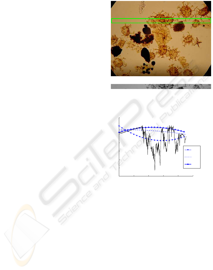
Figure 1: The original image of palynofacies and a grey

stripe cut along the x-axis.

0 500 1000 1500 2000 2500

100

120

140

160

180

(1)

(2)

(3)

image pixels

Grey level intensity

Figure 2: Grey level intensity of the mean line and the three

subsequently ﬁtted parabolas for the stripe in Figure 1.

To exclude the foreground points, a second

parabola is ﬁtted, denoted z

(2)

(x), using a reduced set

of points on the mean line



(x) > z

(1)

(x)

. By

requiring that the grey level intensity exceeds z

(1)

(x),

the most “certain” foreground pixels are eliminated

from the approximation. The resultant parabola

(2)

(x) is shown in Figure 2 with a dashed line. A

third iteration is carried out in the same way, this time

using the set



(x) > z

(2)

(x)

to derive z

(3)

(x)

(triangle maker in Figure 2). It was found empirically

that three iterations give a sufﬁciently good result.

(iii) Consider pixel (x,y) with grey level inten-

sity p(x,y). Let the pixel be in the i-th horizontal

stripe and j-th vertical stripe. The pixel is labelled as

VISAPP 2008 - International Conference on Computer Vision Theory and Applications

140

foreground (object) iff

p(x,y) <

(3)

(x) − T

, z

(3)

(x) − T

, (2)

where T

and T

are automatically calculated thresh-

olds as explained later. Otherwise the pixel is la-

belled as background. In other words, the point must

be classed as foreground in both horizontal and ver-

tical directions in order to receive a ﬁnal label as

foreground. The segmented image is obtained by la-

belling all pixels in the image in this way.

3 EXPLANATION OF THE

METHODOLOGICAL AND

PARAMETER CHOICES

I. The choice of two one-dimensional models instead

of a joint quadratic model was based on empirical

observation. The segmentation accuracy of the

joint quadratic model appeared to be compromised

for some images, arguably because of the coarse

approximation.

II. The decision to divide the image into

stripes was dictated by the large computational

demand should each horizontal and vertical

line be processed in turn. We found empir-

ically that K

= ceiling(No. Rows/40) and

= ceiling(No. Columns/40) is a good com-

promise between accuracy and speed.

III. The need to combine the horizontal and

vertical labelling with an “and” operation (equivalent

to making the decision by equation (2)) is explained

below. Some images contain a large proportion of

objects located at the centre. This may cause the

parabola to be a trough rather than a hill even after the

third iteration (z

(3)

(x)). Then the edges of the image

will be mislabelled as foreground. It is unlikely

that the same will happen to the orthogonal stripe

that runs across that edge. If a pixel is labelled as

background in that stripe, the overall label assigned

by (2)) will be corrected to “background”. Figure

3 shows the results from applying separately a

horizontal and a vertical approximation. Unwanted

artefacts in the form of skidmarks are present in both

images. Only when a point is labelled as foreground

in both images its overall label will be returned as

“foreground”. It may occur that a single vertical or

horizontal scan produces good enough results, for

instance if the illumination varies from top to bottom

a single horizontal scan could be sufﬁcient. Although

illumination variation in microscopy images is not

usually from top to bottom we have found no loss

of quality by combining two separate scans, even in

these cases.

IV. The thresholds T

and T

are determined automati-

cally from the respective parabolas z

(3)

(x) and z

(3)

(x).

The parabola givesthe “middle” background intensity

in the stripe. However, ﬂuctuations about the curve

may also belong in the background. The following

heuristic threshold T

is proposed for horizontal stripe

= max

(3)

(x) − mean

(3)

(x) (3)

is calculated in the same way for the vertical

stripes. Using the standard deviation of the points or

the maximum residual are additional possibilities for

constructing the thresholds.

4 EXPERIMENTS

The background removal method was applied to

seven microscopy images containing microfossils

similar to Figure 1. This technique takes less than 0.8

s for an image of 758 by 568 pixels when run using

Matlab on a PC with a Pentium-4 3.2-GHz processor

and 2GB of RAM. The following alternative segmen-

tation methods were also tried

1. Thresholding the image with a manually adjusted

constant threshold. Only visual feedback was

used to tune the threshold.

2. Fitting a mixture of two Gaussians on the grey

level histogram and ﬁnding the intensity corre-

sponding to the minimum-error classiﬁcation be-

tween class “background” and “other”. This in-

tensity was used as a threshold across the whole

image. Three Gaussians were also attempted be-

cause the images of interest contain darker and

lighter objects (two foreground classes) and the

background, as seen in Figure 1. Figure 4 illus-

trates this technique. The three ﬁtted Gaussians

are overlaid on the grey level histogram of the im-

age and the threshold (138) is marked with a large

dot. (The thresholds found when two Gaussians

were ﬁtted was 137.)

3. Subtracting the morphological closing of the im-

age from the original and performing a manual

threshold on the result (Gonzalez et al., 2004).

The closing of a greyscale image will suppress

dark regions, masking over the foreground pixels

with intensities of local background pixels. By

subtracting this from the orignal greyscale image

we hope to produce an image of even illumina-

tion, thus allowing a global threshold to be ap-

BACKGROUND SEGMENTATION IN MICROSCOPY IMAGES

141

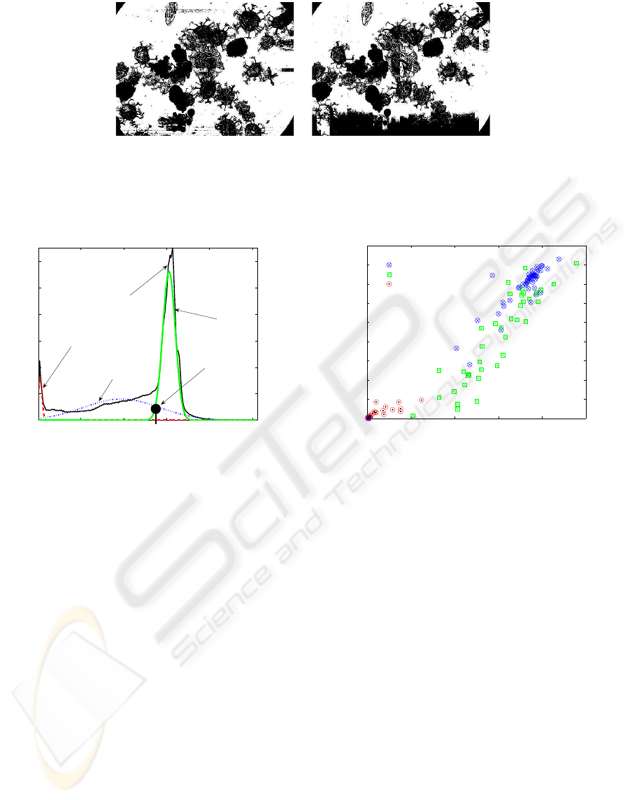
Horizontal scan Vertical scan

Figure 3: Results from applying separately a horizontal and a vertical approximation.

50 100 150 200 250

0.005

0.01

0.015

0.02

0.025

0.03

3 Gaussians

original histogram

background

light objects

dark objects

THRESHOLD

Figure 4: The grey level histogram of the image in Figure 1

and the ﬁtted mixture of three Gaussians. The threshold is

marked with a large dot.

plied. The exact operation of this procedure is de-

cided by a structuring element. The size of this

structuring element will determine which dark re-

gions are masked.

4. Clustering in the original RGB space. Figure 5

shows an example of the results of applying k-

means clustering to a random sample of 150 pixels

from the image in Figure 1. Three clusters were

identiﬁed, corresponding to background, light and

dark objects, and their projection onto the axes

“red” and “green” are displayed. The covariance

matrices of the clusters were estimated and the

pixels in the original image were then labelled

into foreground and background using the Maha-

lanobis distances to the cluster centres. No im-

provement was found when using a larger sample

of pixels.

5. Fitting a quadratic function. As in the proposed

method, three functions were ﬁtted in the same it-

erative way in order to eliminate the effect of fore-

ground pixels on the approximation.

0 50 100 150 200 250

100

120

140

160

180

Background

Light objects

Dark objects

Red

Green

RGB Clusters

Figure 5: Three clusters of pixels in the RGB space, pro-

jected onto the R-G axes.

6. Fitting a B-spline surface. Lindblad and Bengts-

son (Lindblad and Bengtsson, 2001) propose to ﬁt

a B-spline surface using a least squares estimate

to correct the light intensity across the image. A

global threshold is then applied to segment back-

ground from foreground pixels. In this example

we calculated the threshold as in method 3 (ﬁtting

three Gaussians).

The accuracy of the results was evaluated visually

across a collection of images. Figure 7 gives a typi-

cal example of the segmentation results through meth-

ods 1 to 6, the proposed method is show in ﬁgure 8.

Out of the six alternative methods, method 6 showed

the best results. Methods 3 and 5 showed some miss-

ing or partly captured semi-transparent objects corre-

sponding to organic material. These objects are high-

lighted by ellipses and circles in Figure 7. The pro-

posed technique and method 6 extracted these objects

much more adequately.

Given underneath each subplot is the average

computational time from 3 runs of the chosen method

on the same image. The small changes in process-

VISAPP 2008 - International Conference on Computer Vision Theory and Applications

142

Figure 8: (6) PROPOSED: Parabola ﬁt (0.7787s).

ing time for each run was attributed to background

tasks in Windows XP operating system. (The standard

deviations of the processing times were negligible.)

The computational times indicate that the proposed

method offers a good trade-off between accuracy and

speed compared to the alternatives examined in this

study.

The accuracy of method 6 closely matches that of

the proposed method, however we have found that in

certain circumstances the proposed technique is bet-

ter than method 6. We generated 10 non-uniform

backgrounds of size 200 by 200 pixels. For each

background a dark ring was placed in the centre as

a foreground object. The proposed technique and

the B-spline method were both used to segment the

ring from the image. The accuracy was estimated by

calculating the number of pixels misclassiﬁed by the

methods.

Ten rings of constant thickness (30 pixels) with

increasing inner radius were created and placed one

at a time in the centre of the background. The inner

radii of the circles, expressed as a percentage of the

image width, were 5%, 10%, ..., 50%. For images

with inner radius less than 5% to 40%, the proposed

method was better than the B-spline method while at

radii 45% and 50% the B-spline method was better.

Figure 6 demonstrates why the proposed method

works better than the B-spline method. Subplot (a)

shows the generated image with a dark ring. Subplot

(b) shows only the generated background. Subplot (c)

shows the estimated background using B-spline. The

proposed method can also estimate the background

of the generated image; this is shown in subplot (d).

Notice that the foreground has pulled the background

estimate of method 6 towards lower intensity values

however the proposed method ignores these low in-

tensity values creating an adequate background esti-

mate.

5 CONCLUSIONS

A segmentation method is proposed which models

uneven background in microscopy images by a set of

horizontal and vertical parabolas. The method out-

performs ﬁve standard segmentation techniques on a

collection of test images at a competitive computa-

tional speed. This approach is an automated one as

apposed to morphological closing that requires man-

ually selecting a structuring element.

The number of parameters that are tuned for the

proposed method far exceeds those of the standard

methods and this is why a better segmentation is

found. Manual thresholding requires only 1 param-

eter. Fitting three gaussians each with a centre and

standard deviation requires 6 parameters. Fitting a

quadratic function entails tuning 6 parameters for the

coefﬁcients of the function. Clustering in RGB space

uses 27 parameters, each of the three clusters has a

centre in three dimensions and an associated covari-

ance matrix. The covariance matrix contains 9 values

but due to the symmetry only 6 of these are indepen-

dent. The B-spline method uses a mesh of size 5x5 as

the control points for the surface, hence 25 parameters

are used. The proposed method uses 3 coefﬁcients of

a parabola ﬁtted to each mean row and column. In

our example we used 15 parabolas for the horizontal

ﬁt and 19 for the vertical ﬁt, which results in 102 pa-

rameters.

The segmentation offered by the B-spline method

is in most cases as accurate as the one obtained by

the proposed method. However, the proposed method

takes a fraction of the time the B-spline method needs.

ACKNOWLEDGEMENTS

The EPSRC CASE grant Number CASE/CNA/05/18

is acknowledged with gratitude.

REFERENCES

Asada, N., Amano, A., and Baba, M. (1996). Photometric

calibration of zoom lens systems. IEEE International

Conference on Patter Recognition, pages 186–190.

Cinque, L., Foresti, G., and Lombardi, L. (2004). A cluster-

ing fuzzy approach for image segmentation. Pattern

Recognition, 37(9):1797–1807.

Gonzalez, R. C., Woods, R. E., and Eddins, S. L. (2004).

Digital Image Processing Using Matlab. Pearson Ed-

ucation, Inc.

Leong, F., Brady, M., and McGee, J. (2003). Correction of

uneven illumination (vignetting) in digital microscopy

BACKGROUND SEGMENTATION IN MICROSCOPY IMAGES

143

images. Journal of Clinical Pathology, 56(8):619–

621.

Lindblad, J. and Bengtsson, E. (2001). A comparison of

methods for estimation of intensity nonuniformities in

2d and 3d microscope images of ﬂuorescence stained

cells. Proceedings of the 12th Scandinavian Confer-

ence on Image Analysis (SCIA), pages 264–271.

Montage (2002). Baseline background correction.

http:

//montage.ipac.caltech.edu/baseline.html

Otsu, N. (1979). A threshold selection method from gray

level histogram. IEEE Trans. Systems, Man and Cy-

bernetics, 9:62–66.

Sankur, B. and Sezigin, M. (2004). Survey over image

thresholding techniques and quantitative performance

evaluation. Journal of Electronic Imaging, 13(1):146–

165.

Yu, W., Chung, Y., and Soh, J. (2004). Vignetting distor-

tion correction method for high quality digital imag-

ing. 17th International Conference on Pattern Recog-

nition, 3:666–669.

Zawada, D. G. (2003). Image processing of underwater

multispectral imagery. IEEE Journal of Oceanic En-

gineering, 28(4):583–594.

VISAPP 2008 - International Conference on Computer Vision Theory and Applications

144

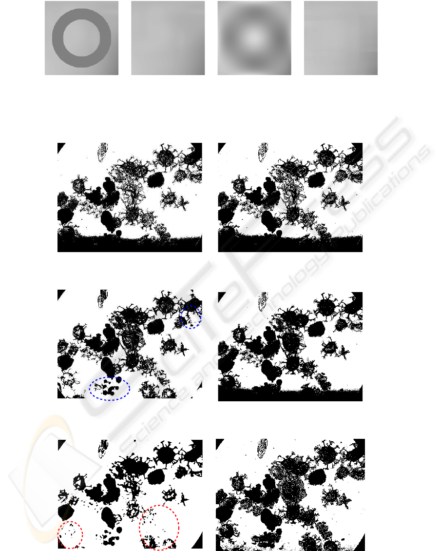
a b c d

Figure 6: (a) Generated image. (b) The true background. (c) The background estimated by the B-spline method. (d) The

background estimated by the proposed method.

(1) Manual thresholding (thr = 135) (2) 3 Gaussians ﬁtted (thr = 138)

(2.6474 s)

(3) Morphological closing (4) Clustering in RGB (3 clusters)

(1.4267 s) (0.8706 s)

(5) Joint quadratic surface (6) B-spline method

(0.2938s) (32.2186 s)

Figure 7: Experimental results: Background removal with the proposed method and the 5 alternative methods.

BACKGROUND SEGMENTATION IN MICROSCOPY IMAGES

145