Adaptive Electrical Signal Post-Processing in Optical

Communication Systems

Yi Sun

, Alex Shafarenko

, Rod Adams

, Neil Davey

Brendan Slater

, Ranjeet Bhamber

, Sonia Boscolo

and Sergei K. Turitsyn

Department of Computer Science, University of Hertfordshire, College Lane

Hatﬁeld, AL10 9AB, U.K.

Photonics Research Group, School of Engineering and Applied Science, Aston University

Birmingham B4 7ET, U.K.

Abstract. Improving bit error rates in optical communication systems is a difﬁ-

cult and important problem. The error correction must take place at high speed

and be extremely accurate. We show the feasibility of using hardware imple-

mentable machine learning techniques. This may enable some error correction at

the speed required.

1 Introduction

Performance of a ﬁbre-optic communication link is typically affected by a complex

combination of random processes (such as ampliﬁed spontaneous emission noise, po-

larization mode dispersion and so on) and deterministic or quasi-deterministic effects

(e.g. nonlinear inter- and intra-channel signal interactions, dispersive signal broaden-

ing, various cross-talks and so on) that result from particular system design and op-

erational regimes. Any installed ﬁbre link has its speciﬁc transmission impairments,

its own signature of how the transmitted signal is corrupted and distorted. Therefore,

there is a great potential in the application of an adaptive signal post-processing that

can undo some of the signal distortions, or to separate line-speciﬁc distortions from

non-recoverable errors. Signal post-processing in optical data communication can offer

new margins in system performance in addition to other enabling techniques. A vari-

ety of post-processing techniques have been already used to improve overall system

performance, e.g. tunable dispersion compensation, electronic equalization and others

(see e.g. [1-4] and references therein). Note that post-processing can be applied both

in the optical and electrical domain (after conversion of the optical ﬁeld into electrical

current). Application of electronic signal processing for compensation of transmission

impairments is an attractive technique that became quite popular thanks to recent ad-

vances in high-speed electronics.

In this work we apply standard machine learning techniques to adaptive signal post-

processing in optical communication systems. To the best of our knowledge this is

the ﬁrst time that such techniques have been applied in this area. One key feature of

this problem domain is that the trainable classiﬁer must perform at an extreme speed,

Sun Y., Shafarenko A., Adams R., Davey N., Slater B., Bhamber R., Boscolo S. and K. Turitsyn S. (2008).

Adaptive Electrical Signal Post-Processing in Optical Communication Systems.

In Proceedings of the 4th International Workshop on Artiﬁcial Neural Networks and Intelligent Information Processing, pages 71-79

DOI: 10.5220/0001507800710079

 SciTePress

optical communication systems typically operate at bit rates of around 40 GHz. We

demonstrate a feasibility of bit-error-rate improvement by adaptive post-processing of

received electrical signal.

2 Background

At the receiver (typically after ﬁltering) the optical signal is converted by a photodiode

into the electrical current. Detection of the digital signal requires discrimination of the

logical 1s and 0s using some threshold decision. This can be done in different ways

(e.g. by considering currents at a certain optimized sample point within the bit time

slots or by analyzing current integrated over some time interval) and is determined

by a speciﬁc design of the receiver. Here without loss of generality we assume that

discrimination is made using current integrated over the whole time slot. Note that the

approach proposed in this paper and described in detail below is very generic and can

easily be adapted to any particular receiver design. To improve system performance

and minimize the bit-error-rate, we propose here to use a method to adjust the receiver

by sending test patterns to transmission impairments speciﬁc for a given line. This is

achieved by applying learning algorithms based on analysis of sampled currents within

bit time slots and adaptive correction of the decisions taking into account accumulated

information gained from analysis of the signal waveforms.

3 Description of the Data

The data represents the received signal taken in the electrical domain after conversion

of the optical signal into an electrical current. The data consists of a large number

of received bits with the waveforms represented by 32 real numbers corresponding to

values of electrical current at each of 32 equally spaced sample points within a bit time

slot. A sequence of 5 consecutive bits is shown in Figure 1. As already explained the

pulse can be classiﬁed according to the current integrated over the width of a single bit.

For each of time slots in our data we have the original bit that it represents. Therefore

the data consists of 32-ary vectors each with a corresponding binary label.

In all we have a stream of 65536 bits to classify. As already explained categorising

the vast majority of these bits is straightforward. In fact with an optimally set electrical

current integrated over the whole time slot (energy threshold) we can correctly classify

all but 1842 bits correctly. We can therefore correctly classify 97.19% of the data, an

error rate of 2.81%. This is however an error rate signiﬁcantly too high. The target error

rate is less than one bit in a thousand, or 0.1%. Figure 2 (a) gives an example of a

misclassiﬁcation. The middle bit of the sequence is a 0 but is identiﬁed from its energy

as a 1. This is due to the presence of two 1

s on either side and to distortion of the

transmitted signal. It would be difﬁcult for any classiﬁer to rectify this error.

However other cases can be readily identiﬁed by the human eye and therefore could

be amenable to automatic identiﬁcation. Figure 2 (b) shows an example where the bit

pattern is obvious to the eye but where a misclassiﬁcation actually occurs. The central

bit is a 1 but is misclassiﬁed as a 0 from its energy alone.

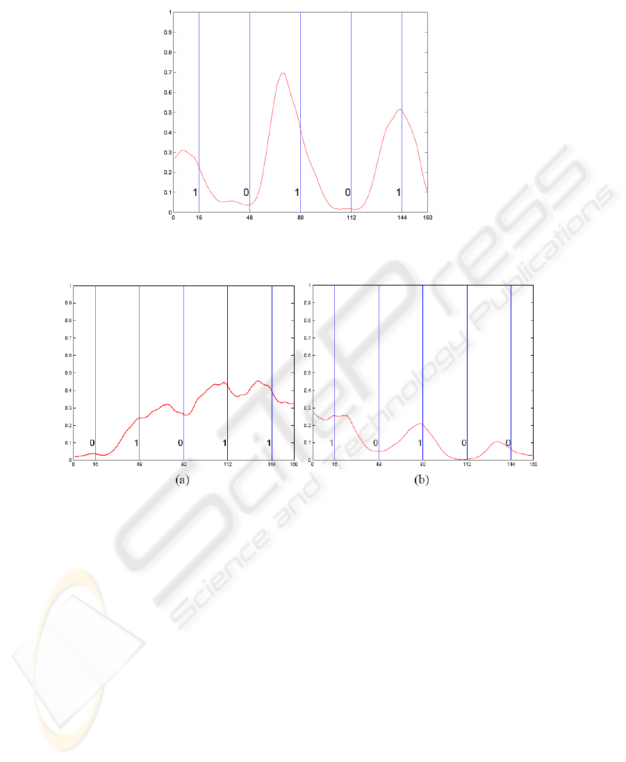
Fig. 1. An example of the electrical signal for a stream of 5 bits - 1 0 1 0 1.

Fig. 2. (a) An example of a difﬁcult error to identify. The middle bit is meant to be a 0, but

jitter has rendered it very hard to see; (b) The central bit has been dragged down by the two 0s

surrounding it and is classiﬁed as a 0 from its energy. However to the human eye the presence of

a 1 is obvious.

3.1 Representation of the Data

Different datasets can be produced depending on how the original electrical current is

represented. As well as representing a single bit as a 32-ary vector (called the Waveform-

1 dataset), it can also be represented as a single energy value (the sum of the 32 values,

Energy-1).

As described above of the 65536 bits, all but 1842 are correctly identiﬁed by an

energy threshold. There are 32 distinct streams of 5 bits and 9 of these are represented

in the misclassiﬁed class with a high frequency from 5.86% to 21.17% among the 1842

misclassiﬁed cases. These nine sequences are shown in Table 1.

Table 1. Nine sequences for which difﬁculties are most likely to occur.

0 0 1 0 0

0 0 1 0 1

0 1 0 1 0

0 1 0 1 1

1 0 0 1 1

1 0 1 0 0

1 0 1 0 1

1 1 0 1 0

1 1 0 1 1

As can be seen the majority of these involve a 1 0 1 or 0 1 0 sequence around

the middle bit, and these are the patterns for which difﬁculties are most likely to occur.

Therefore we may also want to take advantage of any information that may be present

in adjacent bits. To this end we can form windowed inputs, in which the 3 vectors rep-

resenting 3 contiguous bits are concatenated together with the label of the central bit

being the target output (Waveform-3). It is also possible that using adjacent bit infor-

mation by simply taking 3 energy values instead of the full waveform (Energy-3), or

using information from a window of 3 bits, with 1 either side of the target bit (Energy-

Waveform-Energy). Table 2 gives a summary of all the different datasets.

Table 2. The different datasets used in the ﬁrst experiment.

Name Arity Description

Energy-1 1 The energy of the target bit

Energy-3 3 The energy of the target bit and one bit either side

Waveform-1 32 The waveform of the target bit

Waveform-3 96

The waveform of the target bit and the waveforms of the

bits on either side

Energy-Waveform-Energy

(E-W-E)

The waveform of the target bit and the energy of one bit

either side of the target bit

4 Approaches Used

4.1 Easy and Hard Cases

One difﬁculty for the trainable classiﬁer is that in this dataset the vast majority of ex-

amples are straightforward to classify. The hard cases are very sparsely represented, so

that, in an unusual sense, the data is imbalanced. Figure 3 is a diagram of error rates

of 0 and 1 as a function of the energy threshold. It shows that if the energy threshold

is set to roughly 2.5, then those bits with energy less than this threshold are correctly

classiﬁed into the 0 class; on the other hand, if the energy threshold is set to about 11,

then those bits with energy greater than this are correctly classiﬁed into the 1 class. The

optimal energy threshold to separate two classes is 5.01, in which case, 1842 of 65532

are incorrectly classiﬁed - a bit error rate of 2.81%. Using this threshold we divide the

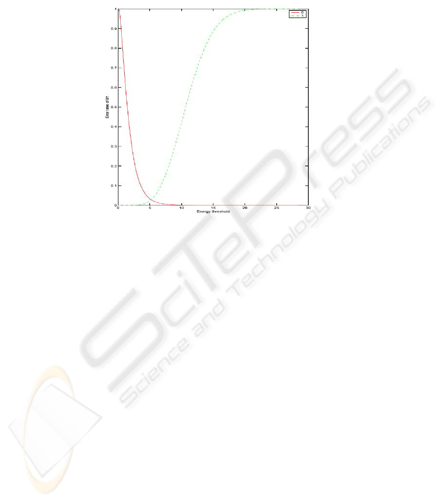
data into easy and hard cases, that is, those classiﬁed correctly by the method are easy

ones, otherwise they are hard cases.

Fig. 3. A diagram of error rates of 0 and 1 as a function of an energy threshold.

4.2 Visualisation using PCA

Before classifying bits into two classes, we ﬁrst look at the underlying data distribution

by means of Classical principal component analysis PCA [5], which linearly projects

data into a two-dimensional space, where it can be visualised.

We visualise the easy cases using PCA, then project the hard cases into the same

PCA projection space. The result is shown in Figure 4 (a). It shows that unsurprisingly

the easy 0 and 1 classes are linearly separable. Interestingly, the hard 0 and 1 classes

are for the most part also linearly separable. However, the hard 1s have almost complete

overlap with the easy 0s, and the hard 0s have almost complete overlap with the easy

1s.

Figure 4 (b) is the eigenwave of the ﬁrst component in the PCA analysis, which

accounts for 86.5% of the total variance.

4.3 Single Layer Neural Network

As already described the classiﬁers need to be operationally very fast. Therefore the

main classiﬁer we use is a simple single layer neural network (SLN) [5]. Once trained

(this is done off-line in advance) an SLN can be built in hardware and function with

great speed. For comparison purposes a classiﬁer that uses just an optimal energy

threshold is implemented, where the threshold is the one giving the maximum accu-

racy rate (97.19%).

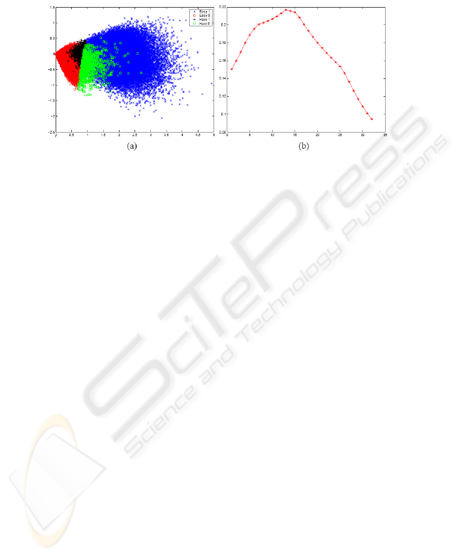
Fig. 4. (a)Projection of the easy set using PCA, where the hard patterns are also projected into the

easy ones’ ﬁrst two principal components space; (b) Eigenwave of the ﬁrst principal component.

4.4 Identifying Difﬁcult Cases using the Energy

As mentioned in Section 4.2, once the hard cases have been separated from the easy

cases, it is possible to linearly separate the 1s and 0s for even the hard cases. Therefore,

the question is how to distinguish between easy and hard cases. One way to tackle the

problem is to use an energy threshold band. So we can set two thresholds, E

min

and

max

, with E

min

≤ E

max

, such that if the energy of a bit is less than E

min

then that

bit is deﬁnitely a 0, and if is greater than E

max

then it is a 1. For those bits whose energy

lies between E

min

and E

max

, they can be considered as difﬁcult cases. Experiment 2

describes how an energy threshold band can be used to select difﬁcult cases which are

subsequently used as training data to an SLN.

4.5 Gaussian Mixture Model (GMM)

Another approach we applied in this work is to use a Gaussian mixture model [5].

Distinguish between easy and hard cases can be performed by modelling the class-

conditional probability p(x|c

) for each easy and hard class ﬁrst, then by calculating

corresponding posterior probabilities using Bayes’ theorem.

Since it is usually insufﬁcient to model the conditional density by a single Gaussian

distribution, we apply a Gaussian mixture model for each class-conditional probability

density. In a Gaussian mixture model, the probability density function of each class

is independently modelled as a linear combination of Gaussian basis functions. The

number of basis functions, their position and variance and their mixing coefﬁcients are

all parameters of the model.

In a Gaussian mixture model, p(x|c

) is of a linear combination of component den-

sities p(x|j, c

), and be written as follows:

p(x|c

) =

p(x|j, c

)P (j) , (1)

where for each component j, we have a Gaussian distribution function

p(x|j, c

) =

(2π)

|Σ

× exp



−

(x − µ

)

−1

(x − µ

)



, (2)

in which case µ

and Σ

are mean and covariance matrix of each component j respec-

tively. P (j) in equation (1) satisﬁes

j=1

P (j) = 1, 0 ≤ P (j) ≤ 1, (3)

which guarantee that p(x|c

) is a valid density function.

The error function is deﬁned as the negative log-likelihood for the dataset given by

E = − ln L = −

n=1

ln p(x

) = −

n=1







p(x

|j, c

)P (j)







. (4)

The expectation-maximisation (EM) algorithm [6] is used to estimate parameters P (j),

, and Σ

of a mixture model for an optimal ﬁt to the training data.

In our experiment, we ﬁrst estimated parameters of each class-condition density

from the training dataset, where the data has been divided into an easy and hard subset

using the optimal energy threshold. Then we reassign the class membership for each

case using Bayes’ theorem, that is

P (c

|x) =

P (c

)p(x|c

)

i=1

P (c

)p(x|c

)

. (5)

Finally two SLNs were trained on these two reassigned classes. For a new test case,

it is given either an easy or difﬁcult class label using eq.(5), then it is forwarded to

the corresponding trained SLN network based on its class membership to give the ﬁnal

discrimination.

5 Experiments

5.1 The First Experiment

We segment the data into 10-fold cross-training/validation sets and one independent

test set. Each distinct segment has 5096 easy cases and 148 hard ones. Therefore, each

training set includes 47196 cases and each validation set has 5244 cases in total; the

independent test set has 12730 easy ones and 362 hard ones. The results reported here

are therefore evaluations on the independent test set and averages over the 10 different

validation sets. The main results are given in Table 3.

The classiﬁers do give an improvement over the optimal energy threshold method

(Energy-1), with the SLN using the Waveform-3 dataset giving the best result. Interest-

ingly the very simple classiﬁer of the SLN/Energy-3 combination nearly decreased the

error rate 42% on both validation and test sets when compared to the optimal threshold

method. This classiﬁer is simply a single unit with 3 weighted inputs.

To examine more closely how a threshold band performs on the waveform-3 dataset

Experiment 2 was undertaken.

Table 3. The results of classifying the different validation and test sets for the different data

representations. We also give the standard deviation for the validation sets.

Dataset

Validation Sets The independent test set

mean errors errors

easy set hard set

mean accuracy

easy set hard set

accuracy

Energy-1 0 148 97.180 0 362 97.23

Energy-3 22 ± 5 64 ± 7 98.366 ± 0.164 59 148 98.419

Waveform-1 22 ± 5 51 ± 5 98.608 ± 0.136 45 122 98.724

Waveform-3 22 ± 5 50 ± 8 98.633 ± 0.139 45 116 98.770

E-W-E 21 ± 6 50 ± 6 98.642 ± 0.140 49 123 98.686

5.2 The Second Experiment

Three different energy threshold bands are used to ﬁlter out the easy cases as discussed

in Section 4.4. An SLN is then applied to each of the resultant difﬁcult sets of size ap-

proximately 16700, 20600 and 24400, respectively. For the test set, above and below the

threshold band, are classiﬁed appropriately, and the rest, the difﬁcult set, are classiﬁed

using the SLN. The results are given in Table 4.

Table 4. The results of classifying the different validation and test sets for each of the threshold

bands. We also give the standard deviation for the validation sets.

Band

Validation Sets The independent test set

mean errors errors

easy set hard set

mean accuracy

easy set hard set

accuracy

2.5 ≤ x ≤ 10.5 23 ± 6 47 ± 5 98.659 ± 0.117 47 113 98.778

2.0 ≤ x ≤ 11.0 23 ± 5 48 ± 5 98.658 ± 0.122 42 114 98.808

2.0 ≤ x ≤ 12.5 22 ± 5 48 ± 5 98.661 ± 0.132 43 115 98.793

It can be seen that in general there is a classiﬁcation improvement in the hard set on

both validation and test sets when compared with results in Table 3. Using a band range

from 2.0 to 11.0 give the best result on the independent test set over all our experimental

results.

5.3 The Third Experiment

In this experiment, we divide the dataset into easy and hard subsets using Gaussian

mixture models as discussed in section 4.5. For each class (easy/hard), we used a two-

gaussian mixture with diagonal covariance matrices. The results are shown in Table

It gives the best mean accuracy on the validation sets in all experiments, but not in

the independent test set.

Table 5. The results of classifying the different validation and test sets. We also give the standard

deviation for validation sets.

Model

Validation Sets The independent test set

mean errors errors

easy set hard set

mean accuracy

easy set hard set

accuracy

2 gmms ‘diag’ 21 ± 4 48 ± 5 98.675 ± 0.126 49 119 98.717

6 Discussion

The fast decoding of a stream of data represented as pulses of light is a commercially

important and challenging problem. Computationally the challenge is in the speed of the

classiﬁer and the need for simple processing. We have therefore restricted our classiﬁer

to be, for the most part, an SLN and the data is either a sampled version of the light

waveform or just the energy of the pulse. Experiment 1 showed that an SLN trained

with the 96-ary representation of the waveform gave the best performance, reducing the

bit error rate from 2.8% to 1.23%. This ﬁgure is still quite high and we hypothesised

that the explanation was the fact that despite the data set being very large, 65532 items,

the number of difﬁcult examples (those misclassiﬁed by the threshold method) was

very small and dominated by the number of straightforward examples. To see if we

could correctly identify a signiﬁcant number of these infrequent but difﬁcult examples

we undertook experiments 2 and 3 .

Although there was a small improvement obtained by using energy threshold band,

further work is needed to determine if there is an optimal band size. Similar results were

obtained by experiment 3.

This is early work and much of interest is still to be investigated, such as repre-

sentational issues of the waveform, threshold band sizes, and other methods to identify

difﬁcult cases.

References

1. Bulow, H. (2002) Electronic equalization of transmission impairments, in. OFC, Anaheim,

CA, Paper TuE4.

2. Haunstein, H.F. & Urbansky, R. (2004) Application of Electronic Equalization and Error

Correction in Lightwave Systems. In Proceedings of the 30th European Conference on Op-

tical Communications (ECOC), Stockholm, Sweden.

3. Rosenkranz, W. & Xia, C. (2007) Electrical equalization for advanced optical communica-

tion systems. AEU - International Journal of Electronics and Communications 61(3):153-

157.

4. Watts, P.M., Mikhailov, V., Savory, S. Bayvel, P., Glick, M., Lobel, M., Christensen, B.,

Kirkpatrick, P., Shang, S., & Killey, R.I. (2005) Performance of single-mode ﬁber links using

electronic feed-forward and decision feedback equalizers. IEEE Photon. Technol. Lett 17

(10):2206 - 2208.

5. Bishop, C.M. (1995) Neural Networks for Pattern Recognition. New York: Oxford University

Press.

6. Dempster, A.P., Laird, N.M, & Rubin, D.B. (1977) Maximum likelihood from incomplete

data via the EM algorithm. J. Roy. Stat. Soc. B, 39 :1–38.