PARTICLE SWARM FEATURE SELECTION FOR
FMRI PATTERN CLASSIFICATION
Timo Niiniskorpi, Malin Bj
¨
ornsdotter
˚
Aberg and Johan Wessberg
Institute of Neuroscience and Physiology, University of Gothenburg, Box 432, SE-405 30 G
¨
oteborg, Sweden
Keywords:
fMRI, Pattern recognition, Feature selection, Particle swarm optimization.
Abstract:
The application of pattern recognition to functional magnetic resonance imaging (fMRI) data enables exiting
possibilities, including mind-reading and brain-machine interfacing. This paper presents a novel brain state
identification approach, which, using an algorithm based on particle swarm optimization (PSO) in conjunc-
tion with a classifier of choice, identifies important brain voxels – thus both maximizing the classification
performance and identifying physiologically relevant areas of the brain. For classifiers, we have investigated
simple multiple linear regression (MLR) with thresholding and linear support vector machines (SVMs). Ap-
plying the PSO algorithm to single-subject, 2D data from a pleasant touch study, originally containing 5650
voxels, voxel subsets of mean size 64.8 and 132.6 voxels with classification accuracies of 73.1% and 77.0%,
respectively for MLR and SMVs, was obtained. Similarly, on group level 3D data from a fingertapping study,
with a total volume of 61078 voxels, a classification score of 83.5% was achieved on 89 voxels using the
linear regression approach. For both datasets, the identified voxels agreed well with both general linear model
T-maps and physiologically expected regions of activation. The PSO is thus effective in the identification of
high-performing voxel subsets for fMRI volume classification, and also provides physiological information
about brain processing related to the experimental conditions. Moreover, the PSO is a user-friendly algorithm,
requiring little input from the user in terms of parameter specification.
1 INTRODUCTION
The identification of instantaneous cognitive states
based on physical measurements has recently proven
not only feasible, but also highly useful to basic neu-
roscience research as well as clinically. It has, for
example, been shown that it is possible to recognize
the spatial pattern of blood flow changes in the brain,
registered using functional magnetic resonance imag-
ing (fMRI) using machine learning techniques (Nor-
man et al., 2006). These methods typically involve
the training of a classifier, such as support vector ma-
chines (SVM; Suykens et al., 2002), to identify and
label patterns of brain activity.
This kind of multivariate analysis, where groups
of voxels are analyzed collectively, have several ad-
vantages over conventional, univariate general linear
model (GLM; Friston et al., 1994) methods, where
each voxel is analyzed individually. Weak informa-
tion contained in single locations can be accumulated
and brain regions that do not individually carry rele-
vant information might do so when jointly analyzed,
and the multivariate approach is thus more sensitive
(Bj
¨
ornsdotter
˚
Aberg and Wessberg, 2008). Moreover,
a trained classifier can be utilized in the identification
of real-time brain states which offers numerous ex-
citing possibilities (see e.g Norman et al., 2006 for a
review).
Due to practical considerations a restricted num-
ber of fMRI volumes (in the order of hundreds) can
be obtained per scanning session. However, the di-
mensionality of fMRI data is exceedingly high (typ-
ically tens of thousands of brain volume voxels per
time unit), warranting feature reduction to alleviate
the curse of dimensionality (Bellman, 1961). Feature
selection, that is, the explicit identification of a lim-
ited number of informative voxels (Blum and Lang-
ley, 1997), allows for both the localization of involved
brain areas and the use of classifiers which can handle
non-linearites.
We therefore propose an approach to fMRI brain
state classification which includes the detection of a
number and combination of voxels that, directly in
conjunction with a classifier, optimally carry informa-
279
Niiniskorpi T., Björnsdotter Åberg M. and Wessberg J. (2009).
PARTICLE SWARM FEATURE SELECTION FOR FMRI PATTERN CLASSIFICATION.
In Proceedings of the International Conference on Bio-inspired Systems and Signal Processing, pages 279-284
DOI: 10.5220/0001535102790284
Copyright
c
 SciTePress

tion relevant to the classification task. This is a no-
table challenge considering the excessive dimension-
ality of whole-volume fMRI data, and any form of
exhaustive search is unfeasible. Stochastic methods,
including evolutionary algorithms (EAs), have been
tried successfully (
˚
Aberg et al., 2008). Particle swarm
optimization (PSO) is a recently developed stochastic
optimization method that has proven excellent in nu-
merous situations. PSO is inspired by naturally oc-
curring phenomena, namely biological swarming be-
havior where virtual particles fly through the problem
space searching for the optimal solution (Kennedy
and Eberhart, 1995). However, the implementation
is substantially less demanding than that of EAs, and
few parameters require specification.
The aim of this study was, consequently, to de-
velop, implement and evaluate a PSO-based fMRI
brain state classification algorithm, specifically de-
signed to efficiently extract a subset of voxels optimal
for the classification task. The algorithm was evalu-
ated on 2D single-subject data from a tactile study, as
well as a 3D motor task, multi-subject dataset.
2 METHODS
2.1 Data Acquisition
A 1.5 Tesla fMRI scanner (Philips Intera, Eind-
hoven, Netherlands) was used for the data acquisi-
tion. Anatomical scans were collected using a high-
resolution T1-weighted anatomical protocol. Func-
tional scans were collected using a BOLD (blood
oxygenation level dependent) protocol with a T2*-
weighted gradient echo-planar imaging sequence.
The scanning planes (6mm thickness) were oriented
parallel to the line between the anterior and poste-
rior commisure and covered the brain from the top of
the cortex to the base of the cerebellum. The experi-
ments were done in accordance with the Declaration
of Helsinki, and the Regional Ethical Review Board
at University of Gothenburg approved the study.
The single-subject dataset was collected in one
healthy human volunteer (female, right-handed; TR
3.0s; 2.3 x 2.3 mm in-plane resolution). 480 volumes
were acquired, containing 25 slices at a spatial reso-
lution of 128 x 128 voxels. During the scans, the ex-
perimenter applied soft brush strokes of length 16cm
in the distal direction on the right thigh, during one
volume. Three volumes of brushing were alternated
with three volumes of rest.
The multi-subject data was acquired from nine
healthy human volunteers (four female, all right-
handed; TR 3.5s; 1.8 x 1.8 mm in-plane resolution).
Data acquisitions were made with three volumes of
fingertapping, where the subjects were instructed to
tap their right hand fingers to the thumb, and three
volumes of rest alternating according to visual cues
for 120 volumes.
All data was motion corrected. In order to com-
pensate for hemodynamic delay, the first of each three
subsequent volumes of stimulus or rest was omitted
and an average was formed from the remaining two,
resulting in a total of 160 volumes the tactile stimu-
lation, and 40 volumes per individual for the finger-
tapping. For comparision, a standard general linear
model analysis was performed on spatially smoothed
(6mm Gaussian kernel) data (Friston et al., 1994).
In the tactile, single-subject dataset the 2D slice
(5650 voxels) containing the secondary somatosen-
sory cortex, highly involved in the processing of
tactile stimulations, was extracted (Olausson et al.,
2002). The fingertapping data was transformed to
standard MNI-space. From the resulting 91 slices, the
20 most dorsal, containing the primary motor cortex
and supplementary motor area, were extracted. The
subject data was then pooled, resulting in a dataset
containing 360 volumes and 61078 voxels.
The resulting data was randomly divided into
three sets: 70% in the training set, and 15% each in
the test and validation sets. In all datasets there were
equal numbers of each category, and the classification
task was distinguishing between stimulus (fingertap-
ping or brushing) and rest. The training dataset was
used for particle fitness computation, whereas the per-
formance over the iterations was monitored using the
testing data. The final classification performance re-
sult was computed on the validation data, using the
particle with the highest performance on the testing
data.
For data visualization, the program MRIcron
(by Chris Rorden, www.sph.sc.edu/comd/rorden/
mricron/) was used, and all subsequent analysis
was implemented in Matlab (The Mathworks, Mas-
sachusetts, USA).
2.2 Particle Swarm Optimization
Particle swarm optimization (PSO) is a stochastic
optimization method (Kennedy and Eberhart, 1995),
loosely based on the behavior of swarming animals
such as birds and fish. A number of particles, rep-
resenting potential solutions to the problem, are re-
leased in the search space of potential solutions. Each
particle has a position and a velocity, and is free to fly
around the search space. The movement is controlled,
however: the particles accelerate towards the the posi-
tion of the best performing particle as well as towards
BIOSIGNALS 2009 - International Conference on Bio-inspired Systems and Signal Processing
280

each particle’s personal best previous position. The
PSO algorithm, described in table 1, is governed by
a set of rules describing how each particle’s position
and velocity changes over time.
2.2.1 Standard Particle Swarm Optimization
The functions which update each particle’s position
and velocity are fundamentally important. In a stan-
dard PSO with an N-dimensional search space, the
particle velocity (1) and position (2), respectively, are
manipulated thus:
v
id
= w × v
id
+ c
1
× r
1
× (p
id
− x
id
) + c
2
× r
2
× (p
gd
− x
id
)
(1)
x
id
= x
id
+ v
id
(2)
where v signifies the velocity of particle i, x the corre-
sponding position, and d, ranging from 1 through N,
represents the optimization dimension. c
1
is the so-
called cognitive parameter, determining the degree of
acceleration towards the particle’s personal best po-
sition p
id
, and c
2
is a social parameter, determining
the acceleration towards the global best position p
gd
.
w an inertia parameter, regulating the overall rate of
change. The stochastic nature of the velocity equa-
tion is represented by r
1
and r
2
, which are random
numbers in the range [0,1].
To maintain coherence in the swarm, the maxi-
mum velocity is regulated by a parameter v
max
. In
standard PSO implementations, a typical value is
v
max
= |x
max
− x
min
|.
2.2.2 Particle Swarm Optimization for Feature
Selection
In the case of feature selection, the standard PSO must
be modified. The present algorithm is an implemen-
tation of the feature selection method proposed by
Wang et al. (Wang et al., 2007).
Given N as the total number of features, the search
space is binary (any feature is ‘on’ or ‘off’) and N-
dimensional. The particle position represents those
features (voxels) which are selected. In the approach
suggested by Wang et. al., the position is encoded as
a binary array of length N, where a ‘1’ represents that
the corresponding feature is selected, and, conversely,
‘0’ indicates that the feature is not selected. Due to the
excessive dimensionality of fMRI data, however, we
have chosen to sparsely encode particle positions as
arrays of integers containing indices of selected fea-
tures.
The velocity of the particles represents how many
features will be changed from ‘selected’ to ‘not se-
lected’ or vice versa during the update of the position.
The velocity is thus an integer in the range [1, v
max
],
and, in this implementation, the parameter v
max
was
set to N/3.
In accordance with equation 1, the velocity of a
particle is dependent on the distance between two po-
sitions, for example p
id
and x
id
. Let a denote the num-
ber of features that are selected in position p
id
but not
in position x
id
. Let b denote the number of features
that are selected in position x
id
but not in position p
id
.
The distance between these two positions, p
id
-x
id
, is
then expressed as (a − b). Additionally, the velocity
can only be positive, wherefore the absolute value of
the result of equation 1 is taken.
The modified equation for updating a particle’s
velocity in this application is thus:
v
i
= abs(w × v
i
+ c
1
× r
1
× (p
i
− x
i
) + c
2
× r
2
× (p
g
− x
i
))
(3)
However, if the number of features that differs
between the particle’s current position x
i
and the
global best position p
g
is ∆, two different situations
are possible when updating the position with the new
velocity v
i
:
(1) v
i
≤ ∆: v features that differ between x
i
and p
g
will
be selected/unselected. That is, particle i will ‘fly’
towards P
g
in a random manner.
(2) v
i
> ∆: All features in x
i
will be set equal
to P
g
, and v − ∆ features will be randomly se-
lected/unselected. The particle will thus pass by
the global best position and continue exploring the
search space with the velocity v − ∆.
To promote initial exploration of the search space,
and, conversely, convergence and exploitation of
‘good’ neighbourhoods towards the end of an algo-
rithm run, the inertia parameter w is set to decrease
linearly over time according to the following equa-
tion:
w = w
max
− (w
max
− w
min
) ×
iter
iter
max
(4)
where iter is the current iteration and iter
max
is the
maximum number of iterations. The parameters w
max
and w
min
are specified maximum and minimum w-
values respectively.
2.2.3 Fitness Measure
With each iteration, a fitness measure indicating the
goodness of that particular solution, is computed for
each particle as follows:
f
i
(M
c
) =
M
c
M
− εd
c
(5)
PARTICLE SWARM FEATURE SELECTION FOR FMRI PATTERN CLASSIFICATION
281

Table 1: Algorithm for PSO with n particles. x
i
denotes the position for particle i, and v
i
the corresponding velocity.
1. Initialize random positions and velocities for particles, x
i
, v
i
, i = 1...n
2. Evaluate each particle in the swarm, x
i
→ f (x
i
)
3. Update the best position for each particle and the global best position.
- if f (x
i
) > f (p
i
) ⇒ p
i
= x
i
- if f (x
i
) > f (p
g
) ⇒ p
g
= x
i
4. Update velocity and position for each particle, according to equation 1.
5. Return to step 2 unless the termination criterion has been met.
where M
c
is the number of correctly classified pat-
terns out of the total M patterns, d
c
is the average de-
viation for correctly classified samples from the class
labels ‘0’ or ‘1’, and ε is a constant small enough that
a particle with a higher M
c
is always receives higher
fitness than a particle with a lower M
c
. This measure
ensures a good fitness distinction, especially for pat-
terns that are near the separating hyperplane.
For classifiers, we used both linear support vec-
tor machines (Suykens et al., 2002), popularly used
in fMRI classification and simple least squares multi-
ple linear regression with thresholding.
2.2.4 Feature Ranking
In order to reduce the time required for the PSO algo-
rithm to filter out highly irrelevant voxels, a univariate
feature ranking method was employed. For each fea-
ture f
i
a ranking value was calculated thus:
f
i
= abs(
µ
0
− µ
1
σ
0
+ σ
1
) (6)
where µ
0
and µ
1
is the mean value of feature i over
the volumes belonging to class 0 and 1 respectively,
and σ
0
and σ
1
are the standard deviations within each
class. The feature ranking value is thus a measure of
how stable a feature is over the volumes, as well as
how distinctly it can separate the data classes.
The features are ranked accordingly in ascending
order. Any feature i has the following probability P
i
of being selected in the position update function:
P
i
=
n
i
∑
N
i=1
n
i
(7)
given the feature position n
i
, where N is the total num-
ber of features. This approach acts as a mild filter, pri-
oritizing features that are univariately differentiating
yet does not dominate multivariately important vox-
els.
3 RESULTS
All classification results plotted as a function of the
number of PSO algorithm iterations refer to the per-
formance on the testing dataset, which is used to mon-
itor performance over time. All other results repre-
sent the classification performance using the classifier
with the highest performance on the testing dataset as
applied once to the unseen validation dataset. 50%
corresponds to chance. The social and cognitive pa-
rameters of the PSO were empirically set to 2.
3.1 Single-Subject Data
On the individual level 2D tactile data, we applied the
PSO algorithm using both the fast least squares multi-
ple linear regression with thresholding and the slower,
more complex (linear) support vector machines for
classification. The PSO algorithm was applied to the
single-subject dataset 100 times, for 30 iterations of
the algorithm.
The PSO algorithm proved highly successful in
increasing the classification performance on the test-
ing data with both classifiers (see figure 1). How-
ever, where there was a substantial increase in perfor-
mance for the MLR classifier (from 58.1% to 73.3%),
the increase for the SVM-based approach was more
moderate (from 68.4% to 74.2%). At peak perfor-
mance, the MLR achieves similar classification ac-
curacies as the SVM: 73.3% vs. 74.2%. Also, the
MLR appeared to over-train, showing a reduction in
performance at 20 iterations, whereas the SVM gener-
alizes better and reaches a plateau after 10 iterations.
Moreover, the average final feature subset size using
the MLR approach was 64.8 voxels, whereas with the
SVM noticeably more voxels, 132.6, were obtained.
However, the time requirements also differ substan-
tially: the time required for one run is more than 10-
fold longer for SVM (132.8s) than for MLR (12.6s).
On unseen validation data, the percentage correctly
classified volumes was 73.1% for MLR and higher at
77.0% for the SVM.
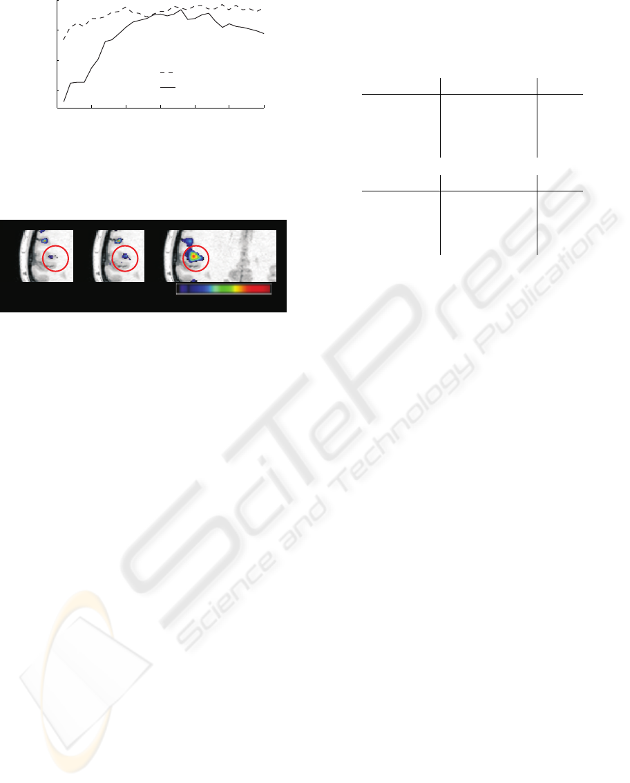
Interestingly, the voxel selection maps, illustrat-
ing the location and selection frequency (in the fi-
BIOSIGNALS 2009 - International Conference on Bio-inspired Systems and Signal Processing
282

Performance (%)
0 5 10 15 20 25 30
65
75
MLR
SVM
70
60
Iteration
Figure 1: Classification performance on the testing data as
a function of the number of PSO algorithm iterations on
the 2D single-subject tactile dataset, using multiple linear
regression (MLR) and support vector machines (SVM).
MLR
SVM
GLM T-map
5 73
Figure 2: The voxel selection maps generated by 100 PSO
iterations on the tactile, single-subject data, and thresholded
to show only outliers. The multiple linear regression-based
classifier (MLR) and support vector machine (SVM) pro-
duce similar maps, and both agree well with the univariate,
standard general linear model (GLM) T-map albeit appear-
ing substantially more specific. The approximate location
of the secondary somatosensory cortex is circled.
nal subset) for individual voxels, generated using both
classifiers differ very little (see figure 2). Both maps
successfully detect the relevant areas (secondary so-
matosensory cortex), but in a much more precise fash-
ion than the standard general linear model T-maps
(thresholded to show significant voxels). The maps
presented here are thresholded to only show voxels
with a selection frequency in the outlier range (larger
than the mean plus six standard deviations).
Table 2 shows a list of the four most selected
outliers presented in the above maps, including the
frequency of selection and univariate feature ranking
score. For both SVM and MLR voxels with low uni-
variate ranks have achieved high selection frequen-
cies, thus indicating that the ranking system does not
influence the feature selection to a degree where the
multivariate feature selection is dominated.
However, disregarding the optimal spatial distri-
bution as achieved with the PSO and including only
these highest ranked voxels in an attempt to classify
the data, substantially lower classification scores were
achieved: 58.3% using MLR and below chance for
the SVM.
Table 2: List of most selected voxels from figure 2. The
lower ranking number, the higher the probability of inclu-
sion of that particular feature in the PSO position update.
The maximum possible selection frequency is 100.
MLR
Feature no. Selection freq. Rank
2183 20 30
2184 15 200
2249 14 179
1727 8 315
SVM
Feature no. Selection freq. Rank
2183 46 30
2248 28 22
2182 22 7
2502 22 118
3.2 Multi-Subject Data
On the whole-volume fingertapping, multi-subject
data, the PSO algorithm in combination with the MLR
was also successful in identifying highly relevant vox-
els. Despite the substantially larger voxel pool (61
078 vs. 5650 voxels), excellent testing data classi-
fication improvement was seen, on average (over 500
runs) increasing from slightly above chance in the first
iteration to near 85% in the last. High classification
scores were achieved with a mean test data perfor-
mance of 83.5% (corresponding mean voxel subset
size of mere 89 voxels), and the resulting validation
data performance was 83.5%.
The cluster of most frequently selected voxels was
located in Brodmann area 4 (Talairach coordinates:
-38 -20 56), containing the primary motor cortex
which is highly involved in the processing of move-
ment.
4 DISCUSSION
This study has successfully implemented an fMRI
pattern classification algorithm, based on particle
swarm optimization, that not only achieves high per-
formance scores but also identifies functionally rele-
vant brain areas. Moreover, the method is easy to use
and requires little parameter specification.
The SVM classifier generally achieved higher
classification results than the MLR, which is expected
since the SVM is a maximum margin classifier with
better (theoretical) generalization. Similarly, feature
selection proved exceedingly important for the simple
linear regression classifier, whereas the support vector
machine, as is well established, handles large dimen-
PARTICLE SWARM FEATURE SELECTION FOR FMRI PATTERN CLASSIFICATION
283

sionalites better. The difference in PSO run time is
more than 10-fold between MLR and SVM, on the
other hand, resulting in a trade-off between classifica-
tion performance and speed of computation. Since the
PSO algorithm is iterative in nature, and thus fairly
computer intensive, the MLR alternative can be pre-
ferred during the feature selection process.
The feature selection frequency maps were thresh-
olded by including only voxels in the outlier range
(figure 2), which does not, naturally, guarantee that
these voxels differ significantly between conditions.
Proper significance thresholding can, however, be
easily performed using non-parametric permutation
testing.
When comparing the feature selection frequency
with the univariate feature ranking (figure 2), it can
be seen that, with both classifiers, roughly the same
features have a high selection frequency. These are
all located in an area that is consistent with the known
anatomical location of the secondary somatosensory
cortex, as confirmed by the general linear model T-
map. Moreover, the voxel selection maps (figure
2) appear virtually identical, and it can thus be as-
sumed that, for multivariate activation localization, ei-
ther SVM or MLR can be used with similar results.
Also, if maximal classification scores are required,
the SVM can be applied on the final selected voxel
subset.
The most frequently selected voxels, however, do
not have the highest ranking values (table 2), showing
that univariate ranking of the features influences but
does not dominate the feature selection process.
The low scores achieved when using only the out-
lier voxels as input into a classifier, indicates that
high-scoring subsets must contain a large variety of
features, including some specific key voxels. These
key voxels appear essential to high accuracy discrim-
ination of conditions, but are poor as individual pre-
dictors. The key voxels can be identified by repeti-
tions of the PSO-algorithm, and subsequent investi-
gation of the feature selection frequency. This is evi-
dence for a distributed nature of brain activation pat-
terns, where optimal voxel subsets may include fea-
tures that, when analyzed individually, do not indicate
any significant difference between conditions. More-
over, this prompts the need for multivariate feature
selection allowing for distributed voxel subsets.
5 CONCLUSIONS
Our proposed particle swarm optimization approach
is effective for fMRI pattern classification, and, more-
over, warrants a user-friendly implementation. Also,
the algorithm can be used to localize voxels that are
highly involved in processing of given conditions.
Simple and fast multiple linear regression approach
appears suitable for the localization of relevant vox-
els, whereas for situations where high-accuracy clas-
sification is required SVMs are highly recommended.
ACKNOWLEDGEMENTS
This study was supported by the Swedish Research
Council (grant K2007-63X-3548) and the Sahlgren-
ska University Hospital (grant ALFGBG 3161). We
are grateful to L. L
¨
oken and K. Rylander for supply-
ing the fMRI data.
REFERENCES
˚
Aberg, M. C., L
¨
oken, L., and Wessberg, J. (2008). An evo-
lutionary approach to multivariate feature selection for
fMRI pattern analysis. Proceedings of the Interna-
tional Conference on Bio-inspired Systems and Signal
Processing.
Bellman, R. E. (1961). Adaptive Control Processes. Prince-
ton University Press, Princeton, NJ.
Bj
¨
ornsdotter
˚
Aberg, M. and Wessberg, J. (2008). An evolu-
tionary approach to the identification of informative
voxel clusters for brain state discrimination. IEEE
Journal of selected Topics in Signal Processing, ((in
press)).
Blum, A. and Langley, P. (1997). Selection of relevant fea-
tures and examples in machine learning. Artificial In-
telligence, 97(1-2):245–271.
Friston, K. J., Holmes, A. P., Worsley, K. J., Poline, J. P.,
Frith, C. D., and Frackowiak, R. S. J. (1994). Statisti-
cal parametric maps in functional imaging: A general
linear approach. Human Brain Mapping, 2(4):189–
210.
Kennedy, J. and Eberhart, R. (1995). Particle swarm opti-
mization. Proceedings of IEEE International Confer-
ence on Neural Networks, 4:1942–1948.
Norman, K. A., Polyn, S. M., Detre, G. J., and Haxby, J. V.
(2006). Beyond mind-reading: multi-voxel pattern
analysis of fMRI data. Trends in Cognitive Sciences,
10(9):Pages 424–430.
Olausson, H., Lamarre, Y., Backlund, H., Morin, C., Wallin,
B. G., Starck, G., S.Ekholm, Strigo, I., Worsley, K.,
Vallbo, A. B., and Bushnell, M. C. (2002). Unmyeli-
nated tactile afferents signal touch and project to insu-
lar cortex. Nature Neuroscience, 5(9):900–904.
Suykens, J., Gestel, T. V., Brabanter, J. D., Moor, B. D., and
Vandewalle, J. (2002). Least Squares Support Vector
Machines. World Scientific, Singapore.
Wang, X., Yang, J., Teng, X., Xia, W., and Jensen, R.
(2007). Feature selection based on rough sets and par-
ticle swarm optimization. Pattern Recognition Letters,
28:459–471.
BIOSIGNALS 2009 - International Conference on Bio-inspired Systems and Signal Processing
284