A BATCH LEARNING VECTOR QUANTIZATION ALGORITHM

FOR CATEGORICAL DATA

Ning Chen

GECAD, Instituto Superior de Engenharia do Porto, Instituto Politecnico do Porto

Rua Dr. Antonio Bernardino de Almeida, 431 4200-072 Porto, Portugal

Nuno C. Marques

CENTRIA/Departamento de Informatica, Faculdade de Ciencias e Tecnologia

Universidade Nova de Lisboa Quinta da Torre, 2829-516 Caparica, Portugal

Keywords:

Learning vector quantization, Self-organizing map, Categorical, Batch SOM.

Abstract:

Learning vector quantization (LVQ) is a supervised learning algorithm for data classiﬁcation. Since LVQ is

based on prototype vectors, it is a neural network approach particularly applicable in non-linear separation

problems. Existing LVQ algorithms are mostly focused on numerical data. This paper presents a batch type

LVQ algorithm used for mixed numerical and categorical data. Experiments on various data sets demonstrate

the proposed algorithm is effective to improve the capability of standard LVQ to deal with categorical data.

1 INTRODUCTION

Classiﬁcation is a fundamental task for modeling

many practical applications, e.g., credit approval,cus-

tomer management, image segmentation and speech

recognition. It can be regarded as a two-stage pro-

cess, i.e., model construction from a set of labeled

data and class speciﬁcation according to the retrieved

model. Kohonen’s learning vector quantization algo-

rithm (LVQ) (Kohonen, 1997) is a supervised vari-

ant of the algorithm for self-organizing map (SOM)

that can be used for labeled input data. Both SOM

and LVQ are based on neurons representing proto-

type vectors and use a nearest neighbor approach for

clustering and classifying data. So, they are neural

network approaches particularly useful for non-linear

separation problems. LVQ can be seen as a special

case of SOM, where the class labels associated with

input data are used for training. The learning pro-

cess tends to perform the vector quantization starting

with the deﬁnition of decision regions and repeatedly

repositing the boundary to improve the quality of the

classiﬁer. In real decision applications, LVQ is usu-

ally combined with SOM (Solaiman et al., 1994), ﬁrst

generating a roughly ordered map through SOM and

then ﬁne tuning the prototypes to get better classiﬁca-

tion through the competitive learning of LVQ.

Existing LVQ algorithms are mostly focused on

numerical data. In this paper, the idea of the proposed

algorithm originates from NCSOM (Chen and Mar-

ques, 2005), a batch SOM algorithm based on new

distance measurement and update rules in order to ex-

tend the usage of standard SOMs to categorical data.

In the present study, we advance the methodology of

NCSOM to the batch type of learning vector quantiza-

tion. We call this method BNCLVQ, performing clas-

siﬁcation task on mixed numeric and categorical data.

In one batch round, the Voronoi set of each map neu-

ron is computed by projecting the input data to its best

matching unit (BMU), then the prototype is updated

according to incremental learning laws depending on

class label and feature type. Experiments show that

the algorithm is as accurate as current state-of-the-art

machine learning algorithms on various data sets.

The remaining of this paper is organized as fol-

lows. Section 2 reviews the related work. Section 3

presents a batch LVQ algorithm to handle numeric

and categorical data during model training. In sec-

tion 4, we evaluate the algorithm on some data sets

from UCI repository. Lastly, the contributions and fu-

ture improvements are given in section 5.

2 RELATED WORK

Data could be described by features in numeric and

categorical (nominal or ordinal) types (Chen and Mar-

Chen N. and C. Marques N. (2009).

A BATCH LEARNING VECTOR QUANTIZATION ALGORITHM FOR CATEGORICAL DATA.

In Proceedings of the International Conference on Agents and Artiﬁcial Intelligence, pages 77-84

DOI: 10.5220/0001661700770084

 SciTePress

ques, 2005). Let n be the number of input vectors, m

the number of map units, and d the number of vari-

ables. Without loss of generality, we assume that the

ﬁrst p variables are numeric and the following d − p

variables are categorical, {α

, α

. . . α

} is the list of

variant values of the k

categorical variable (the nat-

ural order is preserved for ordinal variables). In the

following description, x

= [x

, . . . , x

] denotes the

input vector and m

= [m

, . . . , m

] the prototype

vector associated with the j

neuron. Data projec-

tion is based on the distance between input vectors

and prototypes using squared Euclidean distance on

numeric variables and simple mismatch measurement

on categorical variables (Huang, 1998).

d(x

, m

) =

∑

l=1

e(x

, m

) +

∑

l=p+1

δ(x

, m

) (1)

where

e(x

, m

) = (x

−m

)

, δ(x

, m

) =



0 x

= m

1 x

6= m

This distance simply conjoins the usual Euclidean

distance with the number of agreements between cate-

gorical classes. Complementing (Chen and Marques,

2005), this paper will also present how to handle or-

dinal data in BNCLVQ. However care must be taken

so that measures are compatible with the Euclidean

values.

SOM is composed of a regular grid of neurons,

usually in one or two dimensions for easy visualiza-

tion. Each neuron is associated with a prototype or

reference vector, representing the generalized model

of input data. Due to its capabilities in data summa-

rization and visualization, SOM is usually used for

cluster analysis. Through a non-lineartransformation,

the data in high dimensional input space is projected

to the low dimensional grid space while preserving

the topology relations between input data. That is

why resulting maps are sometimes called as topolog-

ical maps. NCSOM is an extension of original SOM

to handle categorical data. It is performed in batch

manner based on the distance measure in Equation (1)

and novel updating rules. Different from traditional

preprocessing approaches, the categorical mapping is

done inside the SOM.

LVQ is a variant of SOM, trained in a supervised

way. The prototypes deﬁne the class regions corre-

sponding to Voronoi sets. LVQ starts from a trained

map with class label assignment to neurons and at-

tempts to adjust the class regions according to labeled

data. In the past decades, LVQ has attracted much at-

tention because of the simplicity and efﬁciency. The

classic online LVQs are studied in literature (Koho-

nen, 1997). In these algorithms, the map units are

assigned by class labels in the initialization and then

updated at each training step. The online LVQs are se-

quential and sensitive to the order of presentation of

input data to the network classiﬁer (Kohonen, 1997).

Some algorithms have been proposed to perform LVQ

in a batch way. E.g., a batch clustering network FK-

LVQ (Zhang et al., 2004) fuses the batch learning,

fuzzy membership functions and kernel-induced dis-

tance measures. FKLVQ is mainly used for clustering

because the learning process is executed in an unsu-

pervised way without the consideration of class label.

It is well known that LVQ is designed for metric

vector spaces in its original formulation. Some ef-

forts were conducted to apply LVQ to nonvector rep-

resentations. For this purpose, two difﬁculties are

considered: distance measurement and incremental

learning laws. The batch manner makes possible to

construct the learning methodology for data in non-

vector spaces such as categorical data. The SOM

and LVQ algorithms in batch version are proposed

for symbol strings based on the so-called redundant

hash addressing method and generalized means or

medians over a list of symbol strings (Kohonen and

Somervuo, 1998). Also, a particular kind of LVQ

is designed for variable-length and feature sequences

to ﬁne tune the prototype sequences for optimal class

separation (Somervuo and Kohonen, 1999).

LVQ is also a viable way to tune the SOM re-

sults for better classiﬁcation and therefore useful in

data mining tasks. In classiﬁcation problems, SOM

is ﬁrstly used to concentrate the data into a small set

of representative prototypes, then LVQ is used to ﬁne

tune the prototypes for optimal separation. It was re-

ported that LVQ is able to improve the classiﬁcation

accuracy of a usual SOM (Kohonen, 1997). Due to

the close relation between SOM and LVQ, the strat-

egy of categorical data processing can be adopted in

LVQ for classiﬁcation tasks.

3 BNCLVQ: A BATCH LVQ

ALGORITHM FOR NUMERIC

AND CATEGORICAL DATA

It is known that batch LVQ beneﬁts from order in-

sensitivity, fast convergence and elimination of learn-

ing rate inﬂuence (Kohonen, 1997). It makes pos-

sible to construct the learning methodology for data

in categorical nonvector spaces. In this section, a

batch LVQ algorithm for mixed numeric and categor-

ical data will be given. Similar to NCSOM, it adopts

the distance measure introduced in previous section.

Before presenting the algorithm, we ﬁrst deﬁne incre-

ICAART 2009 - International Conference on Agents and Artificial Intelligence

mental learning laws that will be used in the proposed

BNCLVQ algorithm.

3.1 Incremental Learning Laws

Batch LVQ uses the entire data for incremental learn-

ing in one batch round. During the training process,

an input vector is projected to the best-matching unit,

i.e., winner neuron with the closest reference vector.

Following (Kohonen, 1997) a Voronoi set can be gen-

erated for each neuron, i.e., V

= {x

| d(x

, m

) ≤

d(x

, m

), 1 ≤ k ≤ n, 1 ≤ j ≤ m} denotes the Voronoi

set of m

. As a result, the input space is separated into

a number of disjointed sets: {V

, 1 ≤ i ≤ m}. At one

training epoch, the Voronoi set is calculated for each

map neuron, composed of positive examples (V

) and

negative examples (V

) indicating the correctness of

classifying. In Voronoi set an element is positive if its

class label agrees with the map neuron, and negative

otherwise. Positive examples fall into the decision re-

gions represented by the corresponding prototype and

consequently make the prototype move towards the

input. While, negative examples fall into other de-

cision regions and consequently make the prototype

move away from the input.

The map is updated by different strategies de-

pending on the type of variables. The update rules

combine the inspiration inﬂuence of positive exam-

ples and suppression inﬂuence of negative examples

to each neuron in a batch round. This is why the

batch type is used here instead of online type. Assume

(t) is the value of the p

unit on the k

feature at

epoch t. Let h

be the indicative function taking 1 as

the value if p is the winner neuron of x

, and 0 other-

wise. Also, s

the denotation function whose value is

1 in case of positive example, and -1 otherwise.

The update rule of reference vectors on numeric

features conducts in the similar way as NCSOM.

Since LVQ is used to tune the SOM result, here the

neighborhood is ignored and the class label is taken

into consideration. If the denominator is 0 or negative

for some m

, no updating is done. Thus, we have the

learning rule on numeric variables:

(t + 1) =

∑

i=1

∑

i=1

(2)

where



1 if p = arg min

j=1

d(x

, m

(t))

0 otherwise



1 if label(m

) = label(x

)

−1 otherwise

As mentioned above, the arithmetic operations are

not applicable to categorical values. Intuitively, for

each categorical variable, the category occurring most

frequently in the Voronoi set of a neuron should be

chosen as the new value for the next epoch. For this

purpose, a set of counters is used to store the frequen-

cies of variant values for each categorical variable,

in a similar way to what was done for NCSOM al-

gorithm. However, we have now taken into account

the categorical information, so the frequency of a par-

ticular category is calculated by counting the number

of positive occurrences minus the number of negative

occurrences in the Voronoi set.

F(α

, m

(t)) =

∑

i=1

v(h

| x

= α

), r = 1, 2, . . . , n

(3)

F(α

, m

(t)) represents an absolute voting re-

garding each value α

. As in standard LVQ algo-

rithm, this change is made to better tune the original

clusters acquired from SOM to the available super-

vised data. For nominal features, the best category

c = max

r=1

F(α

, m

(t)), i.e., the value having max-

imal frequency, is accepted if the frequency is posi-

tive. Otherwise, the value remains unchanged. As a

result, the learning rule on nominal variables is:

(t + 1) =



c if F(c, m

(t)) > 0

(t) otherwise

(4)

Different from nominal variables, the ordinal vari-

ables have speciﬁc ordering of values. Therefore, the

updating depends not only on the frequency of values

also on the ordering of values. The category closest to

the weighted sum of relative frequencies on all possi-

ble categories is chosen as the new value concerning

about the natural ordering of values. So, the learning

rule on ordinal variables is:

(t + 1) = round(

∑

r=1

r∗

F(α

, m

(t))

∑

i=1

) (5)

3.2 Algorithm Description

As mentioned, the BNCLVQ algorithm is performed

in a batch mode. It starts from the trained map ob-

tained in an unsupervised way, e.g., the NCSOM al-

gorithm. Each map neuron is assigned by a class la-

bel with a labeling schema. In this paper the major-

ity class is used based on the distance between pro-

totypes and input for acquiring the labeled map. Af-

terwards, one instance x

is input and the distance be-

tween x

and prototypes is calculated using Equation

(1), consequently the input is projected to the closest

Function v(y | COND) is y whenCOND holds and zero

otherwise.

A BATCH LEARNING VECTOR QUANTIZATION ALGORITHM FOR CATEGORICAL DATA

prototype. After all input are processed, the Voronoi

set is computed for each neuron, composed of posi-

tive examples and negative examples. Then the pro-

totypes are updated according to Equation (2), Equa-

tion (4) and Equation (5), respectively. This training

process is repeated iteratively enough iterations until

the termination condition is satisﬁed. The termina-

tion condition could be the number of iterations or a

given threshold denoting the maximum distance be-

tween prototypes in previous and current iteration. In

summary, the algorithm is performed as follows:

1. Compute the trained and labeled map with proto-

types: m

, i = 1, ..., m;

2. For i = 1..., n, input instance x

and project x

its BMU;

3. For i = 1, ..., m, compute V

and V

for m

(t);

4. For i = 1, ..., m, calculate the new prototype m

(t+

1) for next epoch;

5. Repeat from Step 2 to Step 4 until the termination

condition is satisﬁed.

4 EXPERIMENTS AND RESULTS

The proposed BNCLVQ algorithm is implemented

based on somtoolbox (Kohonen, 2005) in matlab run-

ning Windows XP operating system. We mainly con-

cern about the effectiveness of BNCLVQ in classi-

ﬁcation problems. Eight UCI (Asuncion and New-

man, 2007) data sets are chosen for the following rea-

sons: missing data, class composition (binary class

or multi-class), proportion of categorical values (pure

categorical, pure numeric or mixed) and data size

(from tens to thousands of instances). These data

sets are described in Table 1, including the num-

ber of instances, the number of features (nu:numeric,

no:nominal, or:ordinal), the number of categorical

values (#val), the number of classes (#cla), percent-

age of instances in the most common class (mcc) and

proportion of missing values (mv).

• soybean small data: a well-known soybean dis-

ease diagnosis data with pure categorical variables

and multiple classes;

• mushroom data: a large number of instances in

pure categorical variables (some missing data);

• tictactoe data: a pure categorical data encoding

the board conﬁgurations of tic-tac-toe games, ir-

relevant features with high amount of interaction;

• credit approval data: a good mixture of numeric

features, nominal features with a small number of

values and nominal features with a big number of

values (some missing data);

• heart disease: mixed numeric and categorical val-

ues (some missing data);

• horse colic data: a high proportion of missing val-

ues, mixed numeric and categorical values;

• zoo data: multiple classes, mixed numeric and

categorical values;

• iris data: pure numeric values.

Table 1: Description of data sets.

#features

datasets #ins nu no or #val #cla mcc mv

soybean 47 0 35 0 74 4 36% 0

mushroom 8124 0 22 0 107 2 52% 1.4%

tictactoe 958 0 9 0 27 2 65% 0

credit 690 6 9 0 36 2 56% 1.6%

heart 303 5 2 6 20 2 55% 1%

horse 368 7 15 0 53 2 63% 30%

zoo 101 1 15 0 30 7 41% 0

iris 150 4 0 0 - 3 33% 0

To ensure all features have equal inﬂuence on dis-

tance, numeric features are normalized to unity range.

In our experiments we set termination condition as 50

iterations. For each data set, the experiments are per-

formed in the following way:

1. The data set is randomly divided into 10 folds: 9

folds are used for model training and labeling, and

the remaining is used for performance validation.

2. In each trail, the map is trained with the training

data set in an unsupervised manner by NCSOM

algorithm, and then labeled by the majority class

according to the known samples in a supervised

manner.

3. BNCLVQ is applied to the resultant map in order

to improve the classiﬁcation quality.

4. For validation, each sample of the test data set is

compared to map units and assigned by the label

of BMU. In order to avoid the assignment of an

empty class, unlabeled units are discarded from

classifying. Then the performance is measured by

classiﬁcation accuracy, i.e., the percent of the ob-

servations classiﬁed correctly.

5. Cross-validation is used with 10 random subsam-

ples for computing ﬁnal accuracy average and

standard deviation results.

As other ANN models, LVQ is sensitive to some

parameters in which map size is an important one. In

Table 2, we investigate the effect of map size to the

resulted classiﬁcation precision. Four kinds of maps

are studied for comparison (Kohonen, 2005): ‘mid-

dle’ map is determined by the number of instances

with the side lengths of grid as the ratio of two biggest

ICAART 2009 - International Conference on Agents and Artificial Intelligence

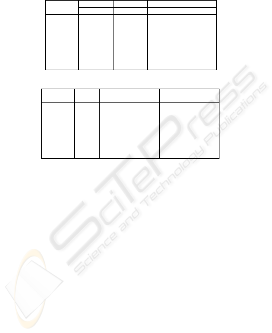
Table 2: Effect of map size to precision.

tiny(%) small(%) middle(%) big(%)

datasets train test train test train test train test

soybean 100 100 100 100 100 100 100 100

mushroom 92 91 96 96 99 98 99 98

tictactoe 73 75 83 75 92 85 95 84

credit 85 83 86 82 89 86 92 85

heart 86 80 86 78 87 82 88 79

horse 83 81 84 84 87 84 90 81

zoo 82 81 90 89 99 99 100 96

iris 95 97 97 96 98 95 99 95

Table 3: Average values of precision and standard deviation.

map train accuracy(%) test accuracy(%)

datasets size NCSOM BNCLVQ NCSOM BNCLVQ

soybean [7 5] 100± 0 100± 2 98± 8 100± 0

mushroom [14 8] 96 ± 1 99± 1 95± 4 98± 3

tictactoe [13 11] 80± 2 92± 1 76 ± 3 85± 3

credit [17 7] 85 ± 1 89± 1 80± 4 86± 3

heart [10 8] 87± 2 87± 2 78± 9 82± 7

horse [11 8] 83± 1 87± 1 79 ± 10 84± 7

zoo [8 6] 99± 1 99± 1 99± 3 99± 3

iris [16 3] 98± 1 97± 1 96 ± 3 95± 3

eigenvalues; ‘small’ map has one-quarter neurons of

‘middle’ one; ‘tiny’ map has half neurons of ‘small’

one; ‘big’ map has four times neurons of ‘middle’

one. As the map enlarges from ‘tiny’ to ‘middle’, both

training precision and test precision improve signiﬁ-

cantly for most data sets (e.g., test precision increases

from 81% to 99% for zoo and 75% to 85% for tic-

tactoe, while soybean and iris are less sensitive to the

change of map size). Further enlarging the map in-

creases the precision in training set, but the test set

precision becomes worse or unchanged, indicating the

map is overﬁtting. It is shown that the maps in mid-

dle size are best for generalization performance ex-

cept on iris data, which achieves desirable precision

using only a ‘tiny’ map of 2 by 2 units. In the follow-

ing experiments, we choose the map of middle size.

As summarized in Table 3, the results show the

potential of BNCLQV compared with NCSOM in im-

proving the accuracy on both training data and test

data for not only data sets of pure categoricalvariables

(e.g., soybean, mushroom and tictactoe) but also those

of mixed variables (e.g., credit, heart, horse and zoo).

Typically, BNCLVQ achieves an increase up to 9%

in classiﬁcation accuracy in tictactoe dataset, when

comparing with using only NCSOM majority class

for classiﬁcation. The results where performance is

almost equivalent are the soybean and iris data sets.

Probably, actually performance on these datasets is

already near reported maximum precisions after run-

ning NCSOM. Also, as it was just veriﬁed in Ta-

ble 2, in BNCLVQ the simpler iris dataset is present-

ing overﬁtting with the ‘middle’ map size (used for

all datasets in this experiment). Performance on BN-

CLVQ networks is always better than the one of NC-

SOM on all datasets without overﬁtting maps. This

gives evidence in favor of the validity of the approach

for reﬁning hybrid SOM maps.

As mentioned previously, SOMs are very useful

for data mining purposes. So, we have also analyzed

our results from the visualization point of view. As

an illustrative example we present the output map for

credit data in Figure 1. Due to the topology preserving

property of SOM, class regions are usually composed

of neighboring prototypes of small u-distance (the

average distance to its neighboring prototypes) val-

ues. The histogram of neurons contains the compo-

sition of patterns presented to the corresponding pro-

totypes. Although neurons of zero-hit have no repre-

sentative capability of patterns, they help to discover

the boundary of class regions. From the visualization

of u-distance and histogram, it becomes easy to de-

tect the separability of classes. Figure 1 shows the u-

distance and histogram chart of trained map for credit

data obtained by NCSOM and BNCLVQ respectively.

Each node has an individual size proportional to its u-

distance value with slices denoting the percentage of

two classes contained. It is observed that BNCLVQ is

able to improve the separation between two class re-

A BATCH LEARNING VECTOR QUANTIZATION ALGORITHM FOR CATEGORICAL DATA

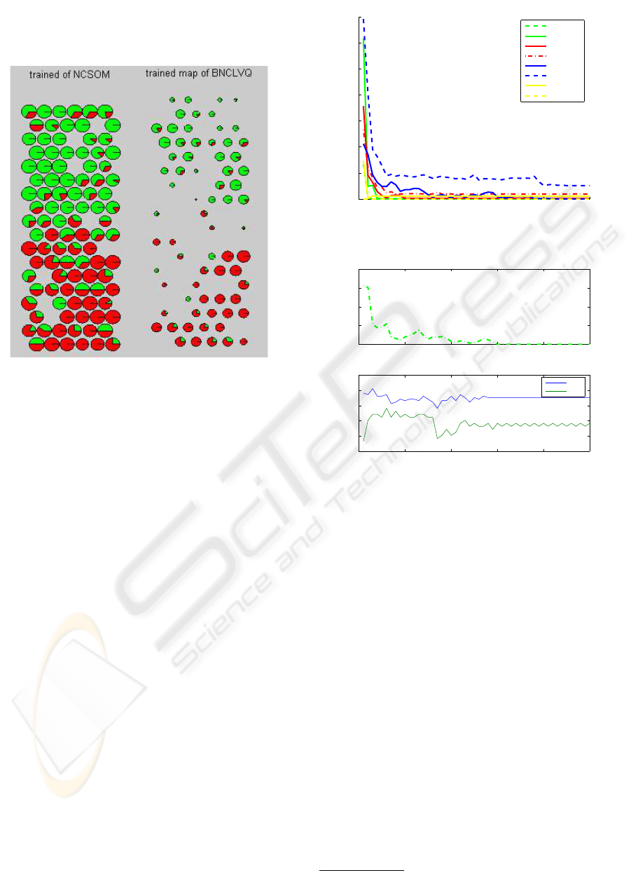
gions (‘approval’ and ‘rejection’) represented by pro-

totypes, showing the capability of BNCLVQ for better

class discrimination.

Figure 1: Histogram visualization on credit data.

We also study the convergence properties of BN-

CLVQ algorithm on the data sets mentioned above.

In this experiment, the convergence was measured as

the overall distance in prototypes between the cur-

rent iteration and the previous iteration: od(t) =

∑

i=1

d(m

(t − 1), m

(t)). As observed in Figure 2 and

Figure 3, the evolution of prototypes reﬂects the sig-

niﬁcant tendency of convergence. The distance de-

creases rapidly in the beginning, and tends to be more

stable after a number of iterations (less than 50 itera-

tions for these data sets). The convergence speed de-

pends on the size of data, number of variables and

speciﬁc properties of data distribution. For example,

it takes only 3 iterations to converge for soybean data.

However for heart data, the variation of prototypes

can be regarded as stable after 30 iterations.

Finally, for better comparison with other ap-

proaches the performance of proposed algorithm is

compared with some representativealgorithms for su-

pervised learning. Six representatives implemented

by Waikato Environment for Knowledge Analysis

(WEKA) (Witten and Frank, 2005) with default pa-

rameters are under consideration:

• Naive Bayes (NB): a well-known representative

of statistical learning algorithm estimating the

probability of each class based on the assumption

of feature independence;

• Sequential minimal optimization (SMO): a sim-

ple implementation of support vector machine

0 10 20 30 40 50

100

200

300

400

500

600

700

number of iterations

overall distance

soybean

mushroom

tictactoe

credit

heart

horse

zoo

iris

Figure 2: Convergence study of BNCLVQ.

0 10 20 30 40 50

100

150

200

number of iterations

overall distance

0 10 20 30 40 50

number of iterations

accuary(%)

train

test

Figure 3: Overﬁtting on heart data.

(SVM). Multiple binary classiﬁers are generated

to solve multi-class classiﬁcation problems;

• K-nearest neighbors (KNN): an instance-based

learning algorithm classifying an unknown pat-

tern to the its nearest neighbors in training data

based on a distance metric (the value of k was

determined between 1 and 5 by cross-validation

evaluation);

• J4.8

: the decision tree algorithm to ﬁrst infer a

tree structure adapted well to training data then

prune the tree to avoid over-ﬁtting;

• PART: a rule-based learning algorithm to infer

rules from a partial decision tree;

• Multi-layer perceptron (MLP): a supervised arti-

ﬁcial neural network with back propagation to ex-

plore non-linear patterns.

We should stress that this comparison may be un-

fair to LVQ. Indeed, as discussed, LVQ is mainly a

projection method that can also be used for classiﬁ-

cation purposes. So, for the sake of comparison, the

A Java implementation of popular C4.5 algorithm.

ICAART 2009 - International Conference on Agents and Artificial Intelligence

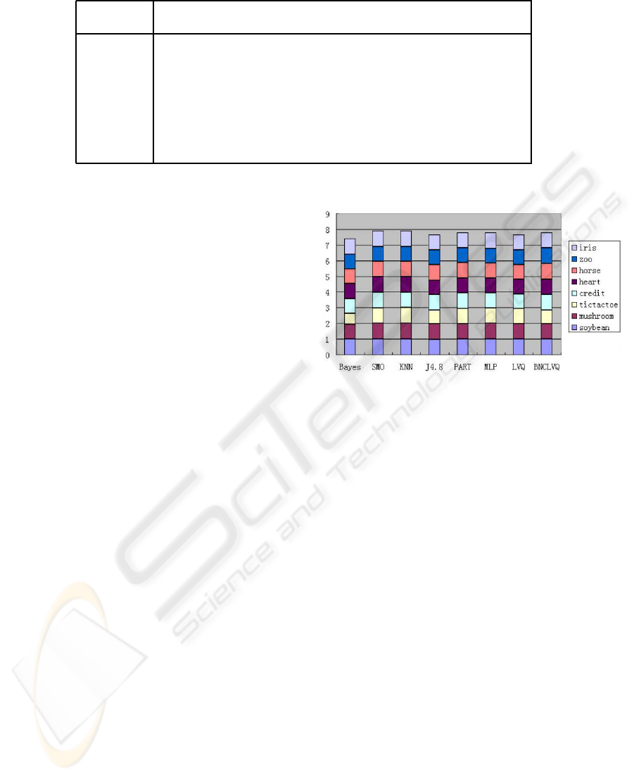
Table 4: Accuracy ratio comparison (the value of k is given for KNN).

Naive SMO BNC

datasets Bayes SVM KNN J4.8 PART MLP LVQ LVQ

soybean 100 100 100(1) 98 100 100 100 100

mushroom 93 99 99(1) 98 98 99 98 98

tictactoe 70 98 99(1) 85 95 97 96 85

credit 78 85 85(5) 86 85 84 80 86

heart 83 84 83(5) 77 80 79 78 82

horse 78 83 82(4) 85 85 80 79 84

zoo 95 93 95(1) 92 92 95 92 99

iris 95 96 95(2) 96 94 97 95 95

standard LVQ is also tested. For doing so, categorical

data are preprocessed by translating each categorical

feature to multiple binary features (i.e., the standard

approach for applying LVQ to mixed datasets).

The summary of results is given in Table 4. For

each data set, the best accuracy is emphasized by

bold. The high-bias performance of naive bayesian

can be explained by the assumption of single proba-

bility distribution (Kotsiantis, 2007). On the contrary,

the other algorithms have high-variance property to

different data sets. Although BNCLVQ is not the best

one for all data sets, it produces desirable accuracy in

most cases, especially on data of mixed types. Also,

BNCLVQ is always better than standard LVQ, the

only exception on tictactoe data is probably caused by

the presence of interaction between features (Stephen,

1999). In (Matheus, 1990), tictactoe original features

were regarded as primary and the inclusion of domain

knowledge and feature generalization improved clas-

siﬁcation accuracyin a very meaningful way. So, BN-

CLVQ seems to be more sensible to some bad encod-

ings of features than standard LVQ. Same pattern is

also observed when comparing J4.8 and PART preci-

sions. This latest result points to some sort of over-

ﬁtting resulting from tictactoe features. Since, like in

decision trees, BCLVQ is a data visualization method,

maybe the same kind of pattern is present. However,

further research needs to be preformed on this dataset

to conﬁrm these hypothesis (Bader et al., 2008).

The robustness of a particular method means how

well it performs in different situations. To compare

the robustness of these classiﬁcation methods, the rel-

ative performance b

on a particular data set is cal-

culated as the ratio of its accuracy and the highest ac-

curacy among all the compared methods (Geng et al.,

2005). A large value of the criterion indicates good

robustness. The robustness distribution is shown in

Figure 4 for each method over the 8 data sets in a

stacked bar. As shown, BNCLVQ achieves a high

summed value only next to SMO and KNN (In fact,

the b

is equal or close to 1 on all the data sets ex-

cept tictactoe), which means BNCLVQ performs well

in different situations.

Figure 4: Robustness of compared methods.

5 CONCLUSIONS

Learning vector quantization is a promising and ro-

bust approach for classiﬁcation modeling tasks. Al-

though originally designed in metric vector spaces,

LVQ could be performed on non-vector data in a

batch way. In this paper, a batch type LVQ algorithm

capable of dealing with categorical data is introduced.

SOM topological maps are very effective tools for

representing data, namely in data mining frameworks.

LVQ is, by itself, a powerful method for classifying

supervised data. Also, it is the most suitable method

to tune SOM topological maps to supervised data.

Unfortunately original LVQ can not handle categor-

ical data in a proper way. In this paper we show

that BNCLVQ is a feasible and effective alternative

for extending previous NCSOM to supervised classi-

ﬁcation on both numeric and categorical data. Since

BNCLVQ is performed on an organized map, only a

limited number of known samples is needed for the

ﬁne-tuning and labeling of map units. Therefore, BN-

CLVQ is a suitable candidate for tasks in which scarce

labeled data and abundant unlabeled data are avail-

able. BNCLVQ is also easy for parallelization (Silva

and Marques, 2007) and can be applicable in frame-

works with very large datasets.

A BATCH LEARNING VECTOR QUANTIZATION ALGORITHM FOR CATEGORICAL DATA

Moreover, BNCLVQ is easily extended to fuzzy

case to solve the prototype under-utilization problem,

i.e., only the BMU is updated for each input (Zhang

et al., 2004), simply replacing the indicative function

by the membership function (Bezdek, 1981). The

membership assignment of fuzzy projection implies

the speciﬁcation to classes, and can be used for the

validity estimation of classiﬁcation (Vuorimaa, 1994).

In the future work, the impact of overﬁtting prob-

lem will be further studied using early stopping strat-

egy on an independent data set and the beneﬁt of

fuzzy strategies in BNCLVQ will be investigated by

cross-validation experiments on both UCI data sets

and state-of-art real world problems. In a ﬁrst real

world case study, we are currently applying NCSOM

topological maps to ﬁne tune mixed numeric and cat-

egorical data in a natural language processing prob-

lem (Marques et al., 2007). In this domain we have

some pre-labeled data available and NCSOM is help-

ing to investigate accurateness and consistency of

manual data labeling. However, already known cor-

rect cases (and possible some previously available

prototypes) should be included in the previously NC-

SOM trained topological map. For that we intend to

use BNCLVQ as the appropriate tool. According to

our results, BNCLVQ can achieve good precision in

most domains. Moreover BNCLVQ is more than a

classiﬁcation algorithm. Indeed BNCLVQ is also a

ﬁne-tuning tool for topological features maps, and,

consequently, a tool that will help the data mining

process when some labeled data is available.

ACKNOWLEDGEMENTS

This work was supported by project C2007-

FCT/442/2006-GECAD/ISEP (Knowledge Based,

Cognitive and Learning Systems).

REFERENCES

Asuncion, A. and Newman, D. J. (2007).

UCI machine learning repository. URL:

http://www.ics.uci.edu/∼mlearn/MLRepository.html.

Bader, S., Holldobler, S., and Marques, N. (2008). Guid-

ing backprop by inserting rules. In d’Avila Garcez,

A. S. and Hitzler, P., editors, Proceeding of 18th Eu-

ropean Conference on Artiﬁcial Intelligence, the 4th

International Workshop on Neural-Symbolic Learning

and Reasoning, volume 366 of ISSN 1613-0073, Pa-

tras, Greece.

Bezdek, J. C. (1981). Pattern recognition with fuzzy objec-

tive function algorithms. Plenum Press, New York.

Chen, N. and Marques, N. C. (2005). An extension of self-

organizing maps to categorical data. In Bento, C., Car-

doso, A., and Dias, G., editors, EPIA, volume 3808 of

Lecture Notes in Computer Science, pages 304–313.

Springer.

Geng, X., Zhan, D.-C., and Zhou, Z.-H. (2005). Su-

pervised nonlinear dimensionality reduction for vi-

sualization and classiﬁcation. IEEE Transactions on

Systems, Man, and CyberneticsCPart B: Cybernetics,

35(6):1098–1107.

Huang, Z. (1998). Extensions to the k-means algorithms

for clustering large data sets with categorical values.

Data Mining and Knowledge Discovery, 2:283–304.

Kohonen, T. (1997). Self-organizing maps. Springer Verlag,

Berlin, 2nd edition.

Kohonen, T. (2005). Som toolbox 2.0. URL:

http://www.cis.hut.ﬁ/projects/somtoolbox/.

Kohonen, T. and Somervuo, P. (1998). Self-organizing

maps of symbol strings. Neurocomputing, 21(10):19–

30.

Kotsiantis, S. B. (2007). Supervised machine learning:

a review of classiﬁcation techniques. Informatica,

31:249–268.

Marques, N., Bader, S., Rocio, V., and Holldobler, S.

(2007). Neuro-symbolic word tagging. In Proceed-

ings of 13th Portuguese Conference on Artiﬁcial In-

telligence (EPIA’07), 2nd Workshop on Text Mining

and Applications, Portugal. IEEE Guimaraes.

Matheus, C. (1990). Adding domain knowledge to sbl

through feature construction. In Proceedings of the

Eighth National Conference on Artiﬁcial Intelligence,

pages 803–808, Boston. MA: AAAI Press.

Silva, B. and Marques, N. C. (2007). A hybrid parallel

som algorithm for large maps in data-mining. In Pro-

ceedings of 13th Portuguese Conference on Artiﬁcial

Intelligence (EPIA’07), Workshop on Business Intelli-

gence, Portugal. IEEE Guimaraes.

Solaiman, B., Mouchot, M. C., and Maillard, E. (1994).

A hybrid algorithm (hlvq) combining unsupervised

and supervised learning approaches. In Proceed-

ings of IEEE International Conference on Neural Net-

works(ICNN), pages 1772–1778, Orlando, USA.

Somervuo, T. and Kohonen, T. (1999). Self-organizing

maps and learning vector quantization for feature se-

quences. Neural Processing Letters, 10(2):151–159.

Stephen, D. B. (1999). Nearest neighbor classiﬁcation from

multiple feature subsets. Intelligent Data Analysis,

3(3):191–209.

Vuorimaa, P. (1994). Use of the fuzzy self-organizing

map in pattern recognition. In Proceedings of the

Third IEEE Conference on Computational Intelli-

gence, pages 478–801.

Witten, H. and Frank, E. (2005). Data mining: practical

machine learning tools and techniques. Morgan Kauf-

mann, San Francisco, 2nd edition.

Zhang, D., Chen, S., and Zhou, Z.-H. (2004). Fuzzy-kernel

learning vector quantization. In Yin, F., Wang, J., and

Guo, C., editors, ISNN (1), volume 3173 of Lecture

Notes in Computer Science, pages 180–185. Springer.

ICAART 2009 - International Conference on Agents and Artificial Intelligence