LINEAR IMAGE REPRESENTATION UNDER CLOSE LIGHTING
FOR SHAPE RECONSTRUCTION
Yoshiyasu Fujita, Fumihiko Sakaue and Jun Sato
Nagoya Institute of Technology, Gokiso-cho, Showa-ku, Nagoya, Japan
Keywords:
Shape from shading, Near light source, Linear representation, 3D shape recovery.
Abstract:
In this paper, we propose a method for representing intensity images of objects illuminated by near point light
sources. Our image representation model is a linear model, and thus, the 3D shape of objects can be recovered
linearly from intensity images taken from near point light sources. Since our method does not require the
integration of surface normals to recover 3D shapes, the 3D shapes can be recovered, even if they are not
smooth unlike the standard shape from shading methods. The experimental results support the efficinecy of
the proposed method.
1 INTRODUCTION
In recent years, the photometric properties of cam-
era image have been studied extensively for recon-
structing 3D shape of objects and for generating pho-
torealistic CG images (Shashua, 1997; Hayakawa,
1994; Mukaigawa et al., 2006; Iwahori, 1990; Kim
and Burger, 1991; Sato et al., 2006; Okabe and Sato,
2006). It has been shown by Shashua (Shashua, 1997)
that if we assume point light source located at infinity
and if there is no specular reflection, we can generate
arbitrary images from the linear combination of three
basis images taken by three different light sources.
Mukaigawa et al. (Y.Mukaigawa et al., 2001) pro-
posed a method called image linearization which en-
ables us to generate arbitrary images from three ba-
sis images, even if specular reflection and/or shadows
exist in images. The photometric properties of each
image point, such as specular reflection, diffuse re-
flection and shadow, can also be classified by using
the image linearization (Mukaigawa et al., 2006).
On the other hand, many method have been pro-
posed for reconstructing 3D shape of objects from im-
age intensities. In general, three or more than three
images are enough for recovering the surface normal
at each image point, and the 3D shape of an object can
be recovered by integrating the surface normal, if the
3D shape is differentiable (Hayakawa, 1994).
Unfortunately, these methods assume that the
point light sources are located at infinity, and they
cannot be applied if the point light sources are close
to the object, i.e. near point light sources. This is
because the images generated by near light sources
include non-linear components, and they cannot be
represented linearly. However, images generated by
near point light source include much more informa-
tion on the 3D geometry than those generated by infi-
nite point light sources, and thus their analysis is very
important.
Iwahori et al. (Iwahori, 1990) proposed a method
for computing surface normal and depth of a Lamber-
tian surface illuminated by a known near light source.
This method solves non-linear equations assuming
that the point light source exists in the direction of
surface normal at a point where the image intensity
is maximum. Kim (Kim and Burger, 1991) analyzed
the uniqueness of the solution to the non-linear equa-
tions. Although these methods enable us to recover
less ambiguous shape information, they require large
computational cost and may not provide us optimal
solutions.
For avoiding these problems, Sato et al. (Sato
et al., 2006; Okabe and Sato, 2006) proposed a
method for linearizing images with near light sources
by dividing the images into small sub-images and as-
suming parallel light in these sub-images. However,
the computational costs of these methods are also
large, since they require iterative algorithm. Further-
more, the accuracy of recovered geometry is not so
good, since only the local constraints are used in each
sub-image.
In this paper, we propose a method for linearly
representing images with near light source. We show
that linear representation of a near point light source
67
Fujita Y., Sakaue F. and Sato J. (2009).
LINEAR IMAGE REPRESENTATION UNDER CLOSE LIGHTING FOR SHAPE RECONSTRUCTION.
In Proceedings of the Fourth International Conference on Computer Vision Theory and Applications, pages 67-72
DOI: 10.5220/0001797000670072
Copyright
c
 SciTePress

image is possible without dividing the image into sub-
images. We also show that the 3D shape of objects
can be recovered directly by using the proposed linear
representation without integrating local surface nor-
mals. Thus, the 3D shape can be recovered accurately,
even if the shape is not smooth. Also, the computa-
tional cost is very small, since the 3D shape can be
recovered linearly by using the proposed linear repre-
sentation.
2 LINEAR REPRESENTATION
OF NEAR LIGHT
SOURCE IMAGES
2.1 Image Representation under Infinite
Light Source
Let us consider a camera, an object and a light source
in the 3D space. In this research, we assume that the
relative position and orientation between the camera
and the object are fixed, and images are taken chang-
ing the position of the light source. We also assume
Lambertian surface for objects in the scene.
Under the assumption of Lambertian surface, the
intensity, I, of the surface can be described by using
the surface normal, n, and the direction of light, s, as
follows:
I = ρE max(n
⊤
s,0) (1)
where, ρ denotes the albedo, and E denotes the in-
tensity of light source. If we assume light source at
infinity, the direction of light source is constant at
any point on the object surface. Thus, if there is no
shadow on the object surface, the whole image of the
object can be represented as follows:
I =








I
1
.
.
.
I
i
.
.
.
I
N








= E








ρ
1
n
⊤
1
.
.
.
ρ
i
n
⊤
i
.
.
.
ρ
N
n
⊤
N








s = EBs (2)
Thus, an image under arbitrary light source can be
described as follows:
I = E[I
1
I
2
I
3
]s
′
= EBAA
−1
s (3)
where, A denotes a 3 × 3 matrix which consists of
three vectors of light direction of I
1
, I
2
and I
3
, and
s
′
= A
−1
s.
As shown in (3), arbitrary images under infinite
light sources can be described linearly by using three
basis images. However, if the light source is close to
the 3D object, the illumination model described in (3)
is no longer valid. In the next section, we consider the
illumination model under near light sources.
2.2 Image Representaion under Near
Light Sources
If the light source is close to the 3D object, the illumi-
nation model described in (3) is no longer valid. If we
consider, the position of the light source, S, a point on
the surface, X, and the surface normal, n, at the point
X, then the image intensity I at the surface point X
illuminated by a near light source S can be described
as follows:
I =
E
||S− X||
2
ρn
⊤
(S− X)
||S− X||
(4)
In (4), (S − X)/||S − X|| describes the direction of
light source, and E/||S− X||
2
corresponds to the at-
tenuation of image intensity according to the distance
between the surface point and the light source.
As shown in (4), we can no longer describe the il-
lumination model linearly, since the direction of light
source at each surface point is not constant, and the
image intensity at a surface point depends on the dis-
tance between the light source and the surface point
as well as the relative orientation between the light
and the surface normal. Thus, the existing methods
require non-linear optimization for recovering the 3D
shape from images taken under near light sources.
2.3 Linear Image Representation under
Near Light Sources
In this section we show a method for linearly repre-
senting images observed under near light sources. We
assume that the attenuation of image intensity caused
by changes in distance between the surface point and
the light source is negligible. This assumption is valid
if the depth of the object is relatively small comparing
with the distance to the object. In this case, the image
intensity I at the surface point X illuminated by a near
light source S can be described as follows:
I = E
ρn
⊤
(S− X)
||S− X||
(5)
Although the direction of light source (S− X)/||S −
X|| is different at each surface point, the position of
the light source S is identical for any surface point. If
we take the square of the image intensity I, we have
I
2
from (5) as follows:
I
2
= ρ
2
E
2
n
⊤
(S− X)n
⊤
(S− X)
(S− X)
⊤
(S− X)
(6)
VISAPP 2009 - International Conference on Computer Vision Theory and Applications
68

Now, let us consider a vector S
2
which consists of
the quadratic terms of S as follows:
S
2
=













S
2
x
S
2
y
S
2
z
S
x
S
y
S
x
S
z
S
y
S
z
S
x
S
y
S
z













(7)
where, S
x
, S
y
and S
z
denote x, y and z coordinates of
the light source position S. Then, (6) can be rewritten
as follows:
λ
e
I
2
= P
e
S
2
(8)
where,
e
I
2
and
e
S
2
represent the homogeneous coordi-
nates of I
2
and S
2
as follows:
e
I
2
=

I
2
1

e
S
2
=

S
2
1

(9)
P is a 2× 10 matrix, which includes the surface nor-
mal and the coordinates of the surface point.
As shown in (8), images taken under near light
sources can be represented linearly by using the
quadratic term of light source position. Since the ma-
trix P includes the shape information of the object,
the 3D shape of the object can be recovered linearly
by using (8). We call P an intensity projection matrix
in the following part of this paper.
2.4 Computing Intensity Projection
Matrix from Images
We next consider a method for computing the inten-
sity projection matrix P from camera images. If we
know the light source position S, the following equa-
tion can be derived by eliminating λ in (8):
h
e
S
2
⊤
−I
2 e
S
2
⊤
i

p
1
p
2

= 0 (10)
where, p
1
and p
2
are ten vector, and P = [p
1
,p
2
]
⊤
.
Thus, if we have M images taken under M differ-
ent light sources, we have the following equation:
M

p
1
p
2

= 0 (11)
where, M is a M × 20 matrix as follows:
M =





e
S
2
1
−I
2
1
e
S
2
1
⊤
.
.
.
f
S
2
M
−I
2
M
f
S
2
M
⊤





(12)
Thus, p
1
and p
2
can be obtained by simply solving
the linear equation (11). Therefore, if we have 19 or
more than 19 images, we can compute the intensity
projection matrix P. Note, the light sources must be
linearly independent in the 9 vector space S
2
.
2.5 Recovering Light Source
Information
Up to now, we derived a method for computing the in-
tensity projection matrix P in the case where the light
source positions S are available. In this section, we
consider a method for recovering the light source po-
sition S in the case where the intensity projection ma-
trix P is given.
If we have P, then the following equation on S can
be obtained from (8):

p
⊤
1
− I
2
p
⊤
2

˜
S
2
= 0 (13)
Since S is constant for all the points in an image, the 9
vector S
2
can be computed from minimum of 9 points
in the image, and the light source position S can be
recovered.
3 RECOVERING 3D SHAPE
FROM INTENSITY
PROJECTION MATRIX
We next consider a method for recovering the 3D
shape of objects by using the linear representation of
intensity images.
In section 2.4, we showed a method for comput-
ing the intensity projection matrix P. Since the inten-
sity projection matrix P includes the 3D coordinates
X and the surface normal n at each surface point of
objects, we can recover the 3D shape of objects from
P.
From (6) we find that the 10 components of p
2
can
be described as follows:
λp
2
=















1
1
1
0
0
0
−2X
−2Y
−2Z
X
2
+Y
2
+ Z
2















(14)
where, X = [X,Y,Z]
⊤
. Thus, the 3D shape X can be
LINEAR IMAGE REPRESENTATION UNDER CLOSE LIGHTING FOR SHAPE RECONSTRUCTION
69

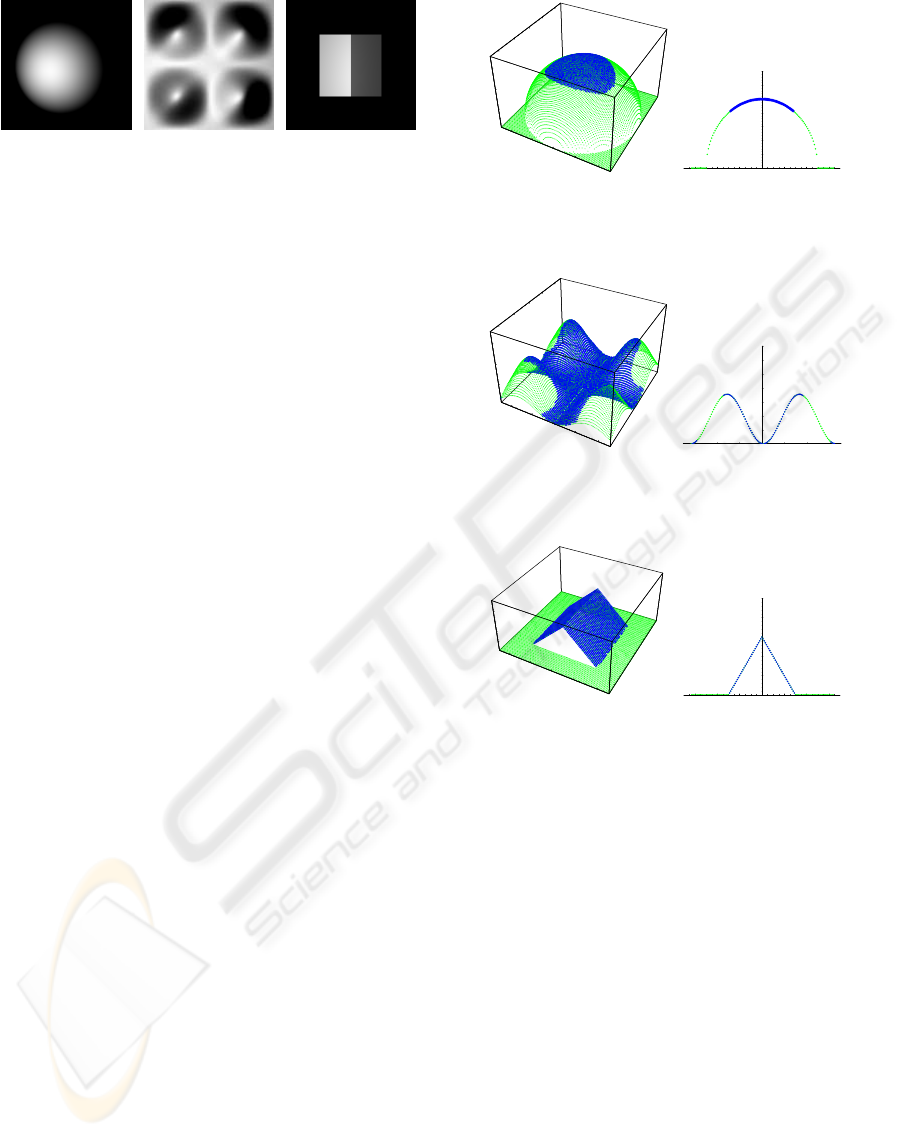
(a) (b) (c)
Figure 1: Example images used in our experiments. (a)
shows the image of a sphere, (b) shows the image of a si-
nusoidal surface, and (c) shows the image of a triangular
prism.
recovered from p
2
as follows:
X =


−p
27
/2p
21
−p
28
/2p
21
−p
29
/2p
21


(15)
where, p
2i
denotes the i-th component of p
2
.
It is known that the standard shape from shading
under infinite light sources can recover the 3D shape
only if the 3D shape is differentiable, since it recovers
the 3D shape by integrating surface normals. How-
ever, the proposed method recovers the 3D shape di-
rectly without using surface normals, and thus it can
recover the 3D shape even if the shape is not smooth.
This is a big advantage of the proposed method to-
gether with the linearity.
4 EXPERIMENTS
We next show the results of some experimentsto show
the efficiency of the proposed method. In these exper-
iments we used synthetic images and evaluated the
proposed method. Fig. 1 shows three example im-
ages used in our experiments, which are images of a
sphere, a sinusoidal surface, and a triangular prism.
The image size is (128× 128).
4.1 Recovery of 3D Shape
We first show the results of recovering 3D shape from
the proposed method. The light source positions are
given in this experiment. The 3D shapes are recov-
ered from 19 images in which the light sources are
close to the objects and are different each other. We
recovered surface points where the image intensities
in 19 images are not equal to 0.
Fig. 2, Fig. 3 and Fig. 4 show the 3D shapes re-
covered by using the proposed method. In these fig-
ures, the blue points show the recovered shapes and
the green points show the ground truth. The RMS er-
rors of the estimated shapes were equal to 0 in all the
shapes. As shown in Fig. 4, the triangular prism can
- 40
- 20
0
20
40
X
- 40
- 20
0
20
40
Y
0
20
40
60
Z
- 40
- 20
0
20
40
X
- 40
- 20
0
20
40
Y
- 60 -40 - 20 20 40 60
X
10
20
30
40
50
60
70
Z
Figure 2: The 3D shape (sphere) recovered by using the pro-
posed method. The blue points show the recovered shape
and the green points show the ground truth.
- 40
- 20
0
20
40
X
- 40
- 20
0
20
40
Y
0
20
40
60
Z
- 40
- 20
0
20
40
X
- 40
- 20
0
20
40
Y
-60 - 40 -20 20 40 60
X
10
20
30
40
50
60
70
Z
Figure 3: The 3D shape (sinusoidal surface) recovered by
using the proposed method. The blue points show the re-
covered shape and the green points show the ground truth.
- 40
- 20
0
20
40
X
- 40
- 20
0
20
40
Y
0
10
20
30
40
50
Z
- 40
- 20
0
20
40
X
- 60 -40 - 20 20 40 60
X
10
20
30
40
50
Z
Figure 4: The 3D shape (triangular prism) recovered by us-
ing the proposed method. The blue points show the recov-
ered shape and the green points show the ground truth. We
find that the proposed method can be applied, even if the 3D
shape is not smooth.
also be recovered accurately, and thus we find that the
proposed method can be applied, even if the 3D shape
is not smooth.
4.2 Generation of Arbitrary Light
Source Images
We next generate arbitrary light source images by us-
ing the proposed linear representation of image inten-
sity. In this experiment, we compute intensity projec-
tion matrix of arbitrary light source positions and gen-
erate synthetic images projecting the recovered 3D
shapes by the intensity projection matrix. The im-
age generation can be achieved linearly by using the
proposed linear representation.
Fig. 5 shows some example images generated by
the proposed method. (a1) and (b1) show synthetic
VISAPP 2009 - International Conference on Computer Vision Theory and Applications
70

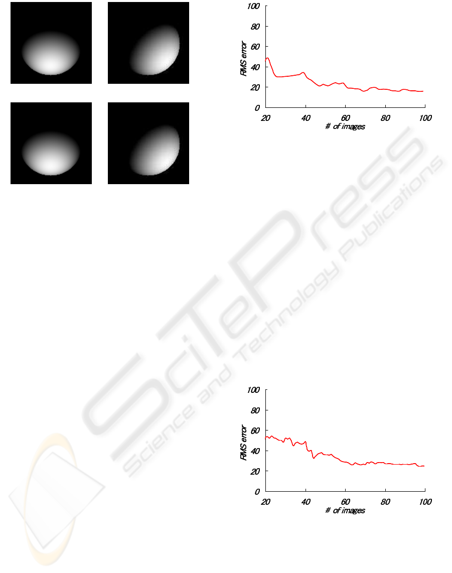
(a1) (b1)
(a2) (b2)
Figure 5: The arbitrary light source images generated by
using the proposed method. (a1) and (b1) show images with
two different light sources, which are generated by using the
intensity projection matrix. (a2) and (b2) show ground truth
images.
images illuminated by two different light sources,
which are linearly generated by using the intensity
projection matrix. (a2) and (b2) show ground truth
images. As shown in this figure, arbitrary light source
images can be generated properly by using the pro-
posed linear representation.
4.3 Accuracy Evaluation under the
Noise in Light Source Positions
We next evaluated the error of the proposed method
caused by the noise in light source positions. In this
evaluation, arbitrary light source images are gener-
ated by using the intensity projection matrix estimated
by adding Gaussian noise with the standard deviation
of 1.0 to all the light source positions. The compu-
tation is iterated 100 times changing the light source
positions, and the RMS errors of generated images are
measured. The same evaluation has been done chang-
ing the number of images used for computing the in-
tensity projection matrix. The results of the evalua-
tion is shown in Fig. 6. As shown in this figure, the
RMS error of generated arbitrary light source images
is going to be small if we use more images for com-
puting the intensity projection matrix.
Figure 6: Accuracy of generated arbitrary light source im-
ages under the noise in light source positions. The hori-
zontal axis is the number of images used for estimating the
intensity projection matrix, and the vertical axis is the RMS
error of generated images.
4.4 Accuracy Evaluation under the
Noise in Images
We finally evaluated the error of the proposed method
caused by the image noise. In this evaluation, we
added Gaussian noises with the standard deviation
of 1.0 to the image intensity, and generated arbitrary
light source images 100 times by using the estimated
intensity projection matrix as before. The RMS er-
rors of generated images are measured changing the
number of images used for computing the intensity
projection matrix. Fig. 7 shows the results of the eval-
uation. As shown in this figure, the proposed method
provides us better results if we use more images for
estimating the intensity projection matrix.
Figure 7: Accuracy of generated arbitrary light source im-
ages under the noise in image intensity. The horizontal axis
is the number of images used for estimating the intensity
projection matrix, and the vertical axis is the RMS error of
generated images.
LINEAR IMAGE REPRESENTATION UNDER CLOSE LIGHTING FOR SHAPE RECONSTRUCTION
71

5 CONCLUSIONS
In this paper, we proposed a method for representing
near light source images linearly. For deriving the lin-
ear representation, we introduced quadratic terms of
a light source position, and the homogeneous repre-
sentation of image intensity is employed. We showed
that the image intensity can be represented linearly by
using the quadratic terms of the light source position.
By using the proposed linear representation, the 3D
shape of objects can be recovered linearly from im-
ages taken under near light sources.
The existing methods of shape from shading can
recover the 3D shape only if the 3D shape is smooth
and differentiable. However, the proposed method re-
covers the 3D shape directly without using surface
normals, and thus it can recover the 3D shape even
if the shape is not smooth. The efficiency of the pro-
posed method was shown in the experiments. The ac-
curacy of the proposed method was also evaluated.
The proposed linear representation of image inten-
sity can be considered as a projective camera projec-
tion from 9D space to 1D space, and thus the proposed
method can be extendedto the case whereboth the po-
sition of light sources and the 3D shape of objects are
unknown by employing the multiple view geometry
in the ordinary cameras.
REFERENCES
Hayakawa, H. (1994). Photometric stereo under a light
source with arbitrary motion. Journal of the Optical
Society of America A, 11(11):3079–3089.
Iwahori, Y. (1990). Reconstructing shape from shading im-
ages under point light source illumination. In Proc.
of International Conference on Pattern Recognition
(ICPR’90).
Kim, B. and Burger, P. (1991). Depth and shape from shad-
ing using the photometric stereo method. CVGIP: Im-
age Understanding, 54(3):416–427.
Mukaigawa, Y., Ishi, Y., and Shakunage, T. (2006). Clas-
sification of photometric factors based on photometric
linearization. Proc. of Asian Conference onf Computer
Vision (ACCV2006), pages 613–622.
Okabe, T. and Sato, Y. (2006). Effects of image segmenta-
tion for approximating object appearance under near
lighting. Proc. of Asian Conference on Computer Vi-
sion (ACCV2006), I:764–775.
Sato, S., Takata, K., and Nobori, K. (2006). Photometric
linearization under near point light sources. IEICE
Trans. Inf. Syst., E89-D(7):2004–2011.
Shashua, A. (1997). On photometric issues in 3d visual
recognition from a single 2d image. International
Journal of Computer Vision, 21:99–122.
Y.Mukaigawa, H.Miyaki, S.Mihashi, and T.Shakunaga
(2001). Photometric image-based rendering for im-
age generation in arbitrary illumination. In Proc.
of International Conference on Computer Vision
(ICCV2001), volume II, pages 652–659.
VISAPP 2009 - International Conference on Computer Vision Theory and Applications
72