EXTRACTING PRINTED DESIGNS AND WOVEN PATTERNS

FROM TEXTILE IMAGES

Wei Jia, Stephen J. McKenna and Annette A. Ward

School of Computing, University of Dundee, Dundee, Scotland, U.K.

Keywords:

Textile segmentation, Pixel labelling, Markov random ﬁeld, Quantitative evaluation.

Abstract:

The extraction of printed designs and woven patterns from textiles is formulated as a pixel labelling problem.

Algorithms based on Markov random ﬁeld (MRF) optimisation and reestimation are described and evaluated

on images from an historical fabric archive. A method for quantitative evaluation is presented and used to

compare the performance of MRF models optimised using α−expansion and iterated conditional modes, both

with and without parameter reestimation. Results are promising for potential application to content-based

indexing and browsing.

1 INTRODUCTION

Accurate automatic extraction of printed designs and

wovenpatterns from images oftextiles is an important

task in providing a suitable representation on which

to build algorithms for the retrieval and browsing of

digital textile archives. This paper discusses colour

segmentation of digital images in a historical com-

mercial archive owned by Liberty Fabric, the fabric

design division of Liberty, London’s iconic depart-

ment store. The Liberty digital archive consists of

many thousands of images, primarily comprising tex-

tile swatches from the past century. Some designs are

printed on the surface of the fabric and other designs

are formed as part of the weave of the fabric. Al-

though many of the images are from the previous 50

years, there are many that are much older, are only

fragments, or have degraded over time; thus adding

complexity to the problem of extraction.

In general the problem of image segmentation is

ill-deﬁned with more than one reasonable segmenta-

tion solution for a given image. Furthermore, many

textile and art images consist of abstract patterns that

make segmentation more challenging. Figure 1(a)

shows a 6-colour design with sketchy ﬂowers and Fig-

ure 1(b) illustrates one possible manual segmentation

of that design into different design components (i.e.,

ﬂowers and leaves).

Formulation of the problem of segmentation of

printed designs and woven patterns requires consider-

ation of textile production. There are various methods

of textile coloration and production. Contemporary

production of Liberty Fabric prints require making a

screen for each colour used in a design. This can be

done by hand tracing or by computer reduction and

separation. Dye is applied to the fabric by ﬂat screens

for short runs and rotary screens for long runs and

continuous designs. However, not all designs in the

archive are printed. Some designs are woven into the

fabric through the weaving process that may be sim-

ple, in the case of stripes, or more complex; for exam-

ple, jacquard.

Figure 1(c-g) shows a ground truth for the origi-

nal image in Figure 1(a) that was obtained by man-

ually assigning its pixels to one of ﬁve classes (i.e.,

colours). However, in a large database, manual label-

ing is not feasible. Thus, the problem to be solved

is to determine the number of classes in a digital tex-

tile image and label each pixel as belonging to one of

these classes. Solutions to this problem can be quanti-

tatively evaluated by comparing computer extractions

with manually-annotated ground-truths such as those

shown in Figure 1(c-g).

Another aspect that may complicate the problem

of segmenting a digital image into colour regions

is the physical surface texture of the fabric (Fig-

ure 2). This is affected by the ﬁbres (e.g., smooth

or crimped), yarns (e.g., soft or hard twist; number

of plies), fabric construction (e.g., type of weave or

knit), and/or textile ﬁnishing (e.g., brushing or chem-

ical application). All of these factors may impact the

visual texture of the image. Methods based on clus-

201

Wei J., J. McKenna S. and A. Ward A. (2009).

EXTRACTING PRINTED DESIGNS AND WOVEN PATTERNS FROM TEXTILE IMAGES.

In Proceedings of the Fourth International Conference on Computer Vision Theory and Applications, pages 201-208

DOI: 10.5220/0001800702010208

 SciTePress

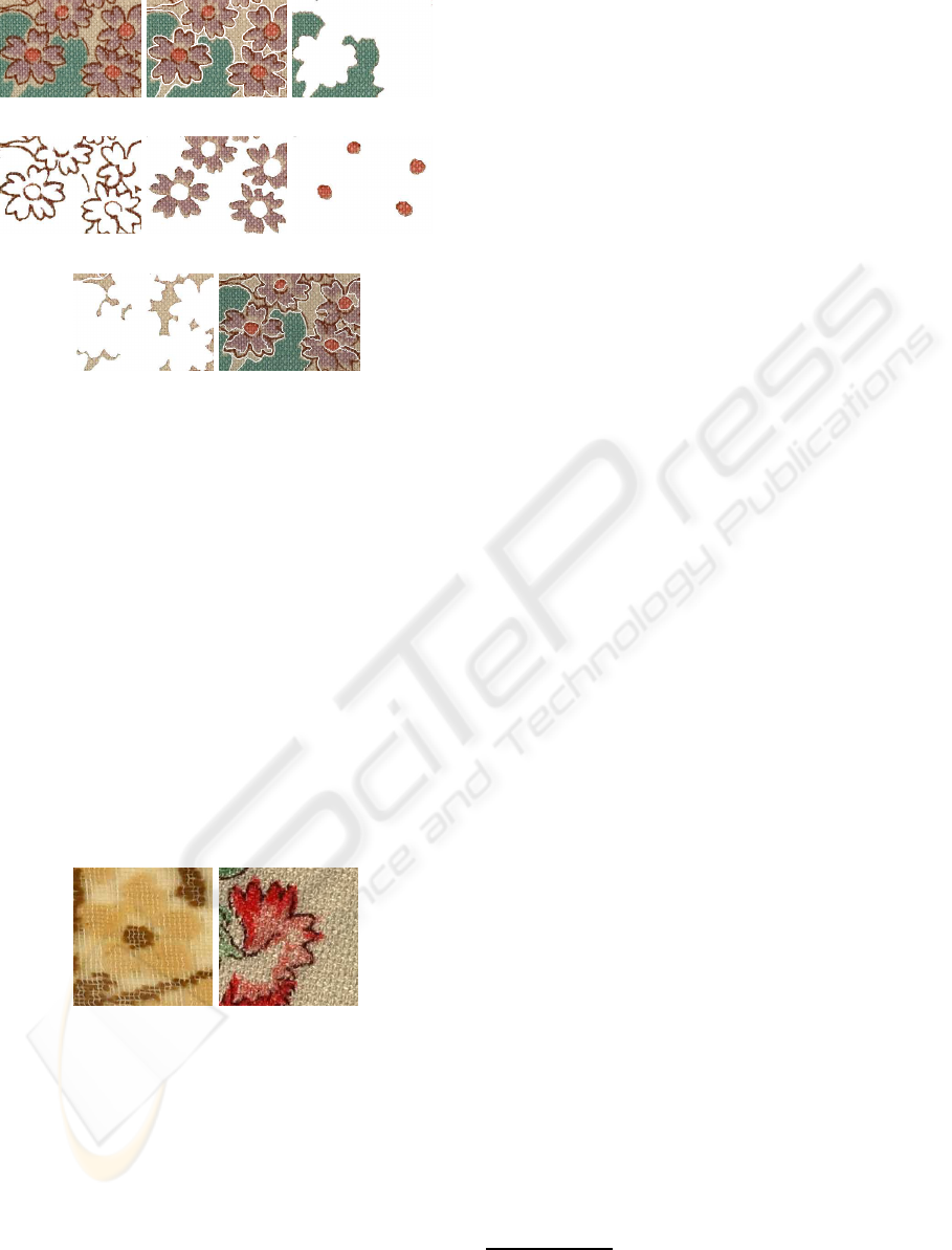
(a) (b) (c) Class 1

(d) Class 2 (e) Class 3 (f) Class 4

(g) Class 5 (h)

Figure 1: (a) A textile image (

Liberty Fabric). (b) One of

many reasonable (manual) segmentations. (c-g) A manually

obtained class labeling of the pixels (h) A JSEG segmenta-

tion.

tering pixels in a colour space without considering the

spatial coherence of the clusters will fail in such cases.

Further difﬁculties arise due to the age and condition

of the textiles, especially in historic archives. For

printed textiles, the saturation of a dye varying within

a region (either due to degradation or by design) may

be problematic. Printing may result in screens being

misaligned and in dyes blending together near their

boundaries to form new colours. However, these ef-

fects are sometimes deliberately introduced to create

additional colour variation or to help ensure that the

fabric is entirely covered with dye leaving no undyed

areas.

(a) (b)

Figure 2: (a) The underlying fabric can be strongly textured.

(b) Colour dyes can blend together and have spatially-

varying density (Images

Liberty Fabric).

Markov random ﬁeld (MRF) models have been

used previously for image segmentation, though usu-

ally for binary foreground-background segmentation

tasks. In this paper, an MRF model is formulated

and applied to the textile segmentation task described

above. Given ground-truth estimates of colour sep-

aration, this application provides a useful test case

for comparing algorithms. A method for quantita-

tive evaluation of multi-class pixel labelling methods

is proposed that handles segmentations with different

numbers of labels. It is used to compare segmentation

results obtained by Gaussian mixture colour cluster-

ing, MRF inference using Iterated Conditional Modes

(ICM), and MRF inference using α−expansion. The

MRF models consider both the class colour distribu-

tions and the spatial coherence of the pixel labels. The

colour distributions are initialised based on a labelling

estimated using a Gaussian mixture in colour space.

The number of colour classes is estimated using the

Bayes Information Criterion (BIC).

Some related work is described in Section 2. The

MRF model along with the algorithms selected to

perform learning and inference are described in Sec-

tion 3. Section 4 describes the evaluation method and

Section 5 reports comparative results obtained using

this method. Finally, Section 6 draws some conclu-

sions and mentions some plans for future work.

2 RELATED WORK

Clustering of local image features or pixel values is

often performed using K-means clustering or Gaus-

sian mixture model (GMM) parameter estimation

with Expectation-Maximisation (EM) (e.g. (Gupta

and Sortrakul, 1998; Wu et al., 2003; Permuter et al.,

2003)). Such clustering treats the features or pixel

values as independent and so when used for segmen-

tation the results often lack spatial coherence, espe-

cially when the images exhibit strong texture. Images

of fabric have been segmented using colour clustering

after ﬁrst attenuating noise and texture by applying

median ﬁltering (Valiente et al., 2001). However, the

use of a median ﬁlter as a preprosessing step can result

in important details being lost. The JSEG segmenta-

tion algorithm (Deng and Manjunath, 2001) performs

colour clustering at the pixel level and then uses re-

gion growing on the cluster labels to segment colour-

texture regions. An example JSEG result is shown

in Figure 1(h)

. Whilst JSEG can ﬁnd reasonable

colour-texture regions, it has two drawbacks. Firstly,

it decomposes the task into two steps of colour clus-

tering and region ﬁnding so that the colour cluster-

ing step takes no account of spatial information. Sec-

ondly, fabric designs have spatially disjoint regions

that share the same colour-texture. We seek a la-

belling that makes this explicit.

The JSEG implementation of Deng and Man-

junath was used with default parameters. See

http://vision.ece.ucsb.edu/segmentation/jseg/

VISAPP 2009 - International Conference on Computer Vision Theory and Applications

202

Markov random ﬁeld (MRF) can provide spatial

constraints in a neighborhood system in the image

domain. They have been used to perform spatially

coherent pixel clustering and promising qualitative

results were reported on two outdoor scenes (Zabih

and Kolmogorov, 2004). Kato and Pong reported

some quantitative segmentation results using an MRF

with pixel colour and local texture features (Kato and

Pong, 2006). However, they assumed that the num-

ber of labels was known. Furthermore, the MRF en-

ergy optimisation methods used by Kato and Pong

no longer represent the state of the art. Compara-

tive studies of MRF optimsation methods on various

computer vision problems have shown methods based

on graph cuts to be effective (Boykov et al., 2001;

Szeliski et al., 2008).

3 MRF SEGMENTATION

Each pixel p is to be assigned a label f

which takes a

value from a discrete label set {1, ...K} with f denot-

ing a particular labelling of all the pixels. The purpose

is to obtain the labelling

f that is most probable given

the image X ,

f = argmax[P( f|X )] = argmax[P(X | f)P( f)] (1)

According to the Hammersley-Clifford theorem

(Li, 1995), the prior probability of a particular la-

belling is:

P( f) ∝ exp(−

∑

( f

, f

)) (2)

where the sum is over all cliques in a neighborhood

system andV

is a clique potential. A clique is deﬁned

as a subset of pixels in the neighborhood system. The

MRFs used in this paper consider adjacent pixel loca-

tions to be neighbours (4-connectivity) and the clique

potentials involve pairs of pixels, so formulation (2)

becomes:

P( f) ∝ exp(−

∑

q∈N

V( f

, f

)) (3)

where q is the neighborhood of p. An important dis-

continuity preserving metric function is given by the

Potts model (Potts, 1952):

V( f

, f

) = λ· (1− δ( f

− f

)) (4)

If labels p and q are different ( f

6= f

) , then its value

is λ. Otherwise its value is zero.

Note that the pixel features are assumed indepen-

dent given the labels, so

P(X | f) =

∏

P(x

| f

) (5)

The likelihood of a label, f

, given its pixel, x

, is

modelled as Gaussian,

P(x

| f

= k) =

exp[−

− µ

)

−1

− µ

)]

(2π)

|Σ

(6)

with parameter set θ

which consists of the mean, µ

and the covariance matrix, Σ

Thus, the problem of segmenting an image is for-

mulated as labelling each pixel with one of K possible

labels and is achieved by minimizing the following

energy function.

E( f) =

∑

q∈N

λ· (1− δ( f

− f

)) −

∑

ln(P(x

| f

)

(7)

where the constant λ ≥ 0 is a coefﬁcient that speciﬁes

the penalty for assigning different labels to neighbor-

ing pixels. Eq. (7) has two terms: the ﬁrst is a smooth-

ing term that rewards spatial coherence and the sec-

ond is a data term.

3.1 Energy Function Minimisation

The energy minimisation problem can be solved by

using the α−expansion algorithm (Szeliski et al.,

2008). The variable α takes values in {1,2,...K} it-

eratively. Within one α−expansion, some of the la-

bels are simultaneously changed to α while all oth-

ers remain unchanged. This gives a new labelling f

which is accepted only if it reduces the energy. In

general there are an exponential number of possible

expansion moves. A graph-based min-cut/max-ﬂow

algorithm (Boykov and Kolmogorov, 2004) has been

used to ﬁnd the optimal expansion move, namely to

ﬁnd the lowest energy within one α−expansion. The

α−expansion algorithm is guaranteed to converge,

terminating when there is no energy decrease for all

values of α.

An alternative and older method, iterated condi-

tional modes (ICM) (Besag, 1986), uses a greedy

strategy to ﬁnd a local minimum of the energy func-

tion. For each pixel in turn, the algorithm chooses the

label which results in the lowest energy. This is re-

peated until convergence. ICM has been reported to

be very sensitive to the initialisation of the labelling.

3.1.1 Initialisation

The number of labels, K, and the initial labelling,

are both estimated using a GMM to model the pixel

values in RGB space. Bayes’ Information Criterion

(BIC) has been found by various authors to give rea-

sonable results when selecting the number of com-

ponents in a Gaussian mixture, e.g. (Roberts et al.,

EXTRACTING PRINTED DESIGNS ANDWOVEN PATTERNS FROM TEXTILE IMAGES

203

1998). Given maximum likelihood parameter esti-

mates

θ , the number of the components is selected

BIC

= argmin

{−L(X|

θ,K) +

M(K)lnN} (8)

where L(X|

θ) is the log likelihood, N is the number

of samples, and M(K) is the number of free param-

eters in the model which in the case of a 3-D GMM

with full covariance matrices is M(K) = (1/2)Kd

(3/2)Kd + K − 1, where d=3. Given the initial la-

belling, the parameters of the class-conditional Gaus-

sians (Eq. 6) are estimated from the pixel data classi-

ﬁed as belonging to that class (using MAP classiﬁca-

tion).

3.1.2 Parameter Re-Estimation

A useful strategy is to alternate energy reduction

and parameter estimation in a manner similar to

Expectation-Maximisation. In the “E” step, the Gaus-

sian parameters are ﬁxed and a new labeling is found.

Given the new labelling, the parameters of the Gaus-

sians are re-estimated conditioned on this labelling

(the “M” step). This results in a new energy func-

tion, the value of which the next “E” step should re-

duce. Since parameter estimation is relatively fast, it

seems reasonable in the case of α−expansion to re-

estimate the Gaussian parameters after each new ex-

pansion step (Zabih and Kolmogorov, 2004).

4 EVALUATION METHOD

Ground-truth labelling can be produced for each im-

age by manual annotation. For visualisation, these la-

bels are mapped to contrasting colours. The accuracy

of an automated labelling is then evaluated by com-

paring it to the ground-truth. However, the label val-

ues are interchangeable. Furthermore, the labelling

obtained will not generally have the same number of

label values as the ground-truth. If two segmenta-

tions use N and M labels respectively then there are

R(M,N) =

(M− N)!

(0 < N ≤ M) possible mappings

between the N labels in one segmentation and the M

labels in the other segmentation. Note thatU = M−N

labels will not ﬁnd a match (U ≥ 0). The measure of

segmentation error which we use is the percentage of

pixels labelled differentlyfrom the ground-truthin the

mapping that minimises this percentage, i.e.,

E = min

100

∑

p=1

δ( f

(1)

− Π( f

(2)

)) (9)

where f

(1)

and f

(2)

are labels assigned to the same

pixel in the two segmentations, and Π denotes a per-

mutation of the labels. Note that labels that do not

ﬁnd a match will contribute to this error. The percent-

age of pixels with unmatched labels will be denoted

U .

(a) (b) (c)

Figure 3: (a) A ground-truth labelling of a 10 × 10 pixel

image. (b-c) Two automatically produced labellings.

Figure 3 shows a simple example for the pur-

poses of illustration. There are R(2,2) = 2 possi-

ble permutations between Figure 3(a) and Figure3(b):



1 → 1

2 → 2



and



1 → 2

2 → 1



where a → b means

label value “a” in labelling 1 corresponds to label

value “b” in labelling 2. Clearly, the latter produces a

lower error. It is this error which is reported. In the

same way, there are R(3,2) = 6 possible permutations

between Figure 3(a) and Figure 3(c). The permutation

that results in the lowest error is:





1 → 3

2 → 2





. In

this case, labels with value “1” in labelling 2 are unas-

signed and so contribute to the error. The accuracy of

the labelling in Figure 3(c) is thus E = 17% of which

U = 13% is attributable to unmatched labels resulting

from incorrect estimation of the number of labels, K.

5 RESULTS AND DISCUSSION

Methods were quantitatively evaluated on images

from a commercial textile archive. The images ranged

in size from 200 × 200 pixels to 2648× 1372 pixels.

These images present challenges to segmentation al-

gorithms as discussed in Introduction. Ground-truth

labellings were produced manually. The test program

was implemented in C and ran on an Intel Core 2

Quad Q6600 2.40GHz PC.

Five methods were evaluated. The ﬁrst method

was Gaussian mixture model clustering using maxi-

mum likelihood EM parameter estimation. Each pixel

was labelled with the most probable Gaussian com-

ponent index conditioned on the pixel’s RGB values.

The second and third methods were MRF labellings

VISAPP 2009 - International Conference on Computer Vision Theory and Applications

204

found using ICM with and without parameter reesti-

mation, denoted ICM and ICM(P) respectively. The

fourth and ﬁfth methods were MRF labellings found

using α−expansion with and without parameter rees-

timation, denoted α and α(P) respectively. The free

parameter in the MRF models was set to λ=6 (see

Eq.(7)) for all images.

Table 1 reports results when the number of labels

was assumed known (i.e., K was the same as in the

ground-truth). Table 2 reports results for the more

difﬁcult (and more realistic) situation in which K was

unknown. The value of K was estimated based on the

BIC values obtained when EM was used to optimise

the parameters of the GMM. The number of colour

dyes used is often limited by production costs in the

type of textile production represented in the data set.

Therefore, very large values of K can be ruled out a

priori. Speciﬁcally, values of K from 1 to 10 were

considered.

Tables 1 and 2 show the errors evaluated us-

ing the method in Section 4 as well as the execu-

tion times. The images, their ground-truth, and seg-

mentations are shown in Tables 3 to 7. In every

case, α−expansion with parameter estimation gave

the lowest error. In many cases ICM with param-

eter estimation performed better than α−expansion

without parameter estimation. This suggests that

parameter reestimation is important for these meth-

ods. GMM gave the highest error. In every case,

α−expansion with parameter reestimation was the

slowest. ICM(P) was slower than ICM, α(P) was

slower than α and GMM was fastest. For each al-

gorithm, computational expense increases with K.

Printing was not always used to create the textiles.

In the textile image in Table 3, there are four differ-

ent colours of ﬁlling yarn (i.e., the yarn that runs hor-

izontally). However, the strong texture and uneven

appearance resulted in BIC estimating K as 7. The

graph plots the BIC value against K. Error bars denote

± a standard deviation (σ) estimated over 10 runs for

each value of K. Segmentation results using K = 4

and K

BIC

= 7 are shown. In both cases, α-expansion

with parameter reestimation is clearly superior.

It is interesting to note that although K was usu-

ally overestimated by BIC, the effect of this on the

segmentation error for α−expansion with parameter

reestimation was not always large. For example, it can

be seen that there is no large difference in error with

different K in Table 3. The α−expansion algorithm

can be understood as a competition between different

labels. In every expansion, α takes one value from

{1,2,...K} and makes some of the pixels become α

simutaneously. If the change is accepted, parameters

will be reestimated, a learning process. This helps

to balance the percentage of different labels. The

ground-truth for the textile image in Table 3 contains

four colours, while K

BIC

= 7, but after α−expansion

with re-estimation only 0.4% of pixels are assigned

labels 5, 6, or 7. Similar comments apply to the tex-

tile images in Table 5 and Table 6. Sometimes, larger

K can help to distinguish similar colors. For exam-

ple, in Table 6, K = 8 is not enough to distinguish

the brown and red colors due to the texture effects

and dye degradation, but K

BIC

= 9 could and gave a

smaller error rate.

In the fabric in Table 7, ﬁlling yarns were inserted

into the warp yarns to create the ﬂoral pattern. Here,

when K = 3, α(P) is superior to the other methods, but

when K

BIC

= 7, although α(P) is better than others, it

loses accuracy.

Tables 4 and 5 show less strongly-textured fab-

rics. Nevertheless, they are problematic. A small

cropped patch of the textile image in Table 5 is shown

magniﬁed in Figure 4(b) where yellow and blue re-

gions overlap and create green. In order to avoid

gaps between different colour regions, two dyes may

be overlapped slightly, thus producing a third colour

and causing difﬁculty for colour segmentation. Fig-

ure 4 graphically illustrates this problem. Figure 4(c)

shows an annotated ground-truth. However, the α-

expansion method separates the overlapping area into

another colour region as shown in Figure 4(d).

6 CONCLUSIONS

In this paper, we have addressed colour separation

of textiles in order to recover printed designs and

woven patterns from archival image data. An eval-

uation method was proposed and used to compare

pixel labellings obtained using MRFs optimised using

α−expansion and ICM both with and without param-

eter reestimation. These algorithms were initialised

based on Gaussian mixture colour models and BIC

was used to select the number of distinct class labels.

For all the images tested, α−expansion with

parameter reestimation was the most accurate

and the most computationally expensive method.

α−expansion without parameter reestimation gave

similar performance to ICM with parameter reesti-

mation. BIC based on GMM usually overestimated

the number of class labels. However, this did not al-

ways result in α−expansion with parameter reestima-

tion obtaining a less accurate result. In fact, in one

case the accuracy was improved.

The pixel labellings produced suggest ways of

compactly representing image content in terms of

colour and shape. Future work will explore their use

EXTRACTING PRINTED DESIGNS ANDWOVEN PATTERNS FROM TEXTILE IMAGES

205

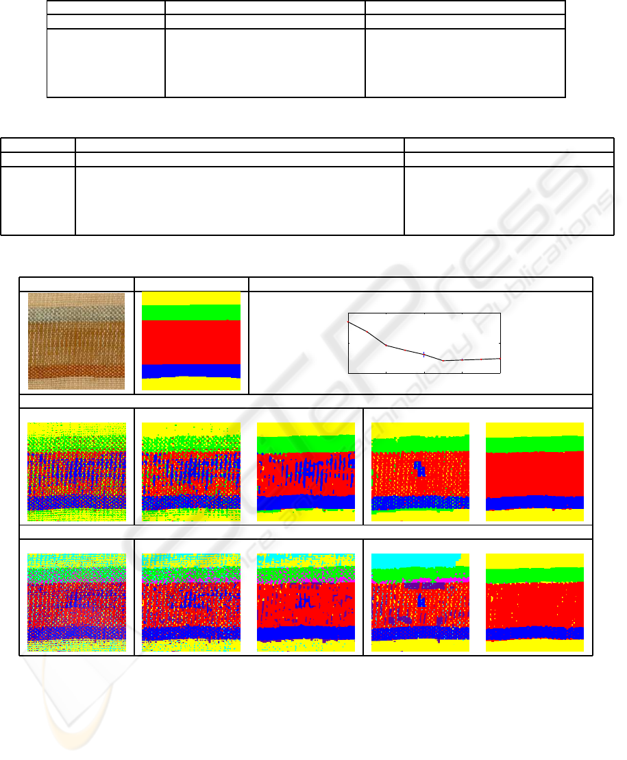
Table 1: Error rates and computing times with known K.

Image Error(%): E Time (s)

Table Size K GMM ICM ICM(P) α α(P) GMM ICM ICM(P) α α(P)

3 200×200 4 39.07 30.85 13.56 11.68 3.30 0.19 0.36 1.14 0.93 1.21

4 1400×544 7 20.85 17.40 15.90 17.04 12.83 7.70 12.93 39.40 50.53 53.76

5 1268×556 7 17.05 14.27 12.23 12.90 6.63 7.02 11.82 36.21 34.21 65.95

6 996×608 8 48.99 42.89 31.56 34.18 24.99 4.97 9.61 33.49 29.11 50.82

7 1594×896 3 25.60 24.00 22.67 23.39 4.65 5.20 10.18 33.09 36.62 55.01

Table 2: Error rates and computing times with K estimated automatically.

Image Error(%): E [U ] Time (s)

Table K

BIC

GMM ICM ICM(P) α α(P) GMM ICM ICM(P) α α(P)

3 7 44.97[30.39] 35.00[25.25] 19.99[17.07] 32.75[27.65] 5.52[0.40] 0.28 0.55 1.87 1.19 2.53

4 7 20.85[0.00] 17.40[0.00] 15.90[0.00] 17.04[0.00] 12.83[0.00] 7.70 12.93 39.40 50.53 53.76

5 9 18.31[9.69] 16.12[9.58] 15.05[9.53] 15.39[9.54] 8.37[4.43] 9.11 15.03 46.13 53.16 100.10

6 9 47.79[6.83] 40.75[5.64] 30.623[9.19] 34.66[8.32] 19.01[0.50] 7.96 12.88 39.49 34.47 63.02

7 7 45.15[44.10] 42.99[42.34] 45.27[44.92] 46.76[46.37] 37.53[36.76] 10.52 20.40 70.44 115.41 190.27

Table 3: Segmentation results on a 200×200 textile image (

Liberty Fabric).

Original ground truth BIC

2 4 6 8 10

4.4

4.6

4.8

x 10

BIC

K = 4

GMM-EM ICM ICM(P) α α(P)

BIC

= 7

GMM-EM ICM ICM(P) α α(P)

in content-based retrieval and browsing.

ACKNOWLEDGEMENTS

The authors wish to thank Anna Buruma and Martin

Coward of Liberty Fabric, and Peter Taylor for help-

ful discussions and advice. This research was sup-

ported by the UK Technology Strategy Board grant

“FABRIC: Fashion and Apparel Browsing for Inspi-

rational Content” in collaboration with Liberty Fab-

ric, System Simulation, Calico Jack Ltd., and the Vic-

toria and Albert Museum. The Technology Strategy

Board is a business-led executive non-departmental

public body, established by the government. Its mis-

sion is to promote and support research into, and de-

velopment and exploitation of, technology and inno-

vation for the beneﬁt of UK business, in order to in-

VISAPP 2009 - International Conference on Computer Vision Theory and Applications

206

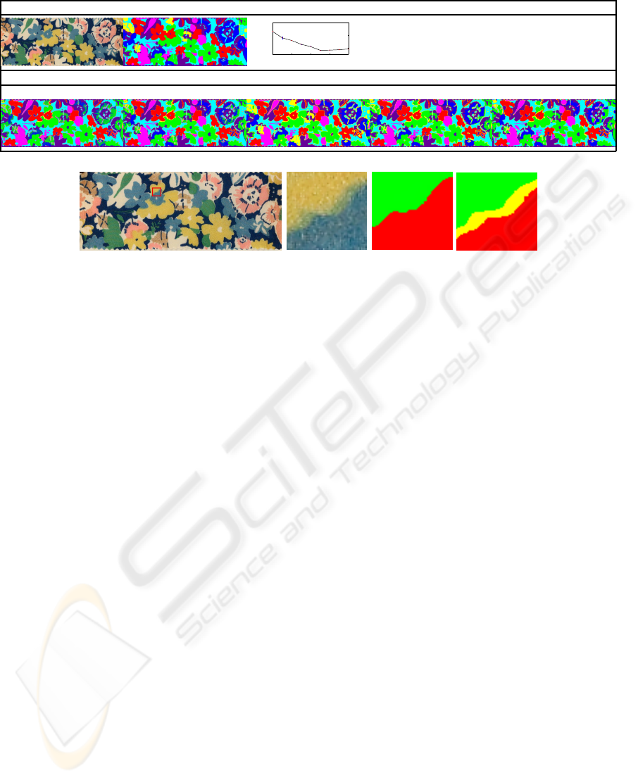
Table 4: Segmentation results on a 1400×544 textile image (

Liberty Fabric).

Original Ground truth BIC

2 4 6 8 10

2.6

2.8

x 10

BIC

K = K

BIC

= 7

GMM-EM ICM ICM(P) α α(P)

(a) (b) (c) (d)

Figure 4: (a) Cropping a small patch of original image (b) Original image patch (c) “Ground truth” (d) α-expansion result.

crease economic growth and improve the quality of

life. It is sponsored by the Department for Inno-

vation, Universities and Skills (DIUS). Please visit:

http://www.innovateuk.org/ for further information.

REFERENCES

Besag, J. (1986). On the statistical analysis of dirty picu-

tures. Journal of Royal Statistical Sociely, Series B,

48(3):259–302.

Boykov, Y. and Kolmogorov, V. (2004). An experimental

comparison of min-cut / max-ﬂow algorithms for en-

ergy minimization in vision. IEEE Transactions on

Pattern Analysis and Machine Intelligence, 26:1124–

1137.

Boykov, Y., Veksler, O., and Zabih, R. (November 2001).

Fast aproximate energy minimization via graph cut.

IEEE Transactions on Pattern Analysis and Machine

Intelligence, 23, no. 11:1222–1239.

Deng, Y. and Manjunath, B. (2001). Unsupervised segmen-

tation of color-texture regions in images and video.

IEEE Transactions on Pattern Analysis and Machine

Intelligence, 23:800–810.

Gupta, L. and Sortrakul, T. (1998). A Gaussian mixture

based image segmentation algorithm. Pattern Recog-

nition, 31(3):315–325.

Kato, Z. and Pong, T. C. (2006). A Markov random ﬁeld

image segmentation model for color texture images.

Image and Vison Computing, 24:1103–1114.

Li, S. Z. (1995). Markov Random Field Modeling in Com-

puter Vision. Springer-Verlag.

Permuter, H., Francos, J., and Jermyn, I. H. (2003). Gaus-

sian mixture models of texture and color for image

database retrieval. Acoustics, Speech and Signal Pro-

cessing, 3:569–572.

Potts, R. (1952). Some generalized order-disorder transfor-

mation. Proc. Cambridge Philosophical Soc., 48:106–

109.

Roberts, S. J., Husmeier, D., Rezek, I., and Penny, W.

(1998). Bayesian approaches to Gaussian mixture

modeling. IEEE Transactions on Pattern Analysis and

Machine Intelligence, 20(11):1133–1142.

Szeliski, R., Zabih, R., Scharstein, D., Veksler, O., Kol-

mogorov, V., Agarwala, A., Tappen, M., and Rother,

C. (2008). A comparative study of energy min-

imization methods for Markov random ﬁelds with

smoothness-based priors. IEEE Transactions on Pat-

tern Analysis and Machine Intelligence, 30:1068–

1080.

Valiente, J. M., Carretero, M. C., Gmis, J. M., and Albert, F.

(2001). Image processing tool for the purpose of tex-

tile fabric modeling. In 12th International Conference

on Designs Tools and Methods.

Wu, Y., Yang, X., and Chan, K. L. (2003). Unsupervised

colour image segmentation based on Gaussian mix-

ture model. Information, Communications and Signal

Processing, 1:541–544.

Zabih, R. and Kolmogorov, V. (2004). Spatially coherent

clustering using graph cuts. IEEE Computer Society

Conference on Computer Vision and Pattern Recogni-

tion, 2:473–444.

EXTRACTING PRINTED DESIGNS ANDWOVEN PATTERNS FROM TEXTILE IMAGES

207

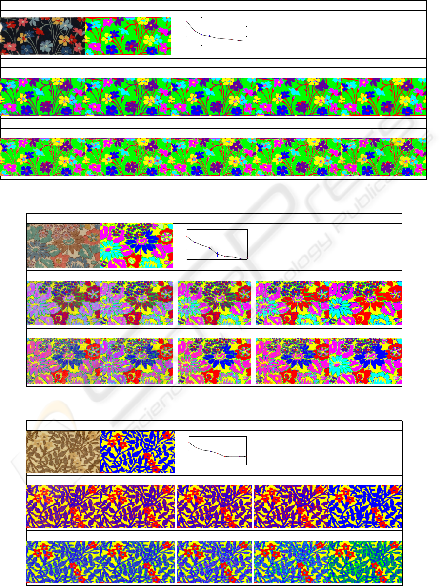
Table 5: Segmentation results on a 1268×556 textile image (

Liberty Fabric) with small texture affection.

Original Ground truth BIC

2 4 6 8 10

1.15

1.2

1.25

1.3

x 10

BIC

K = 7

GMM-EM ICM ICM(P) α α(P)

BIC

= 9

GMM-EM ICM ICM(P) α α(P)

Table 6: Segmentation results on a 996×608 textile image (

Liberty Fabric).

Original Ground truth BIC

2 4 6 8 10

1.25

1.3

1.35

1.4

x 10

BIC

GMM (K = 8) ICM (K = 8) ICM(P) (K = 8) α (K = 8) α(P) (K = 8)

GMM (K

BIC

= 9) ICM (K

BIC

= 9) ICM(P) (K

BIC

= 9) α (K

BIC

= 9) α(P) (K

BIC

= 9)

Table 7: Segmentation results on a 1594×896 textile image (

Liberty Fabric).

Original Ground truth BIC

2 4 6 8 10

1.1

1.15

1.2

x 10

BIC

GMM (K = 3) ICM (K = 3) ICM(P) (K = 3) α (K = 3) α(P) (K = 3)

GMM (K

BIC

= 7) ICM (K

BIC

= 7) ICM(P) (K

BIC

= 7) α (K

BIC

= 7) α(P) (K

BIC

= 7)

VISAPP 2009 - International Conference on Computer Vision Theory and Applications

208