A CAMERA AUTO-CALIBRATION ALGORITHM FOR REALTIME

ROAD TRAFFIC ANALYSIS

Juan Carlos Tocino Diaz, Quentin Houben, Jacek Czyz, Olivier Debeir and Nadine Warz

LISA, Universte Libre de Bruxelles, Avenue Franklin Roosevelt 50 CP165/57, Brussels, Belgium

Keywords:

Camera calibration, Road lane markings, Visual trafﬁc analysis.

Abstract:

This paper presents a new mono-camera system for trafﬁc surveillance. It uses an original algorithm to ob-

tain automatically a calibration pattern from road lane markings. Movement detection is done with a Σ − ∆

background estimation which is a non linear method of background substraction based on comparison and

elementary increment/decrement. Foreground and calibration data obtained allow to determine vehicles speed

in an efﬁcient manner. Finally, a new method to estimate the height of vehicles is presented.

1 INTRODUCTION

Road trafﬁc is increasing each year. Understanding

its characteristics is very helpful to motorway admin-

istrators to cope with this growth, and achieve regula-

tions. Among trafﬁc characteristics, user behaviours

and classes of vehicles are the most relevant.

Until a few years ago, the main measurement tool

for trafﬁc analysis was the magnetic inductive loop.

That kind of sensors has serious drawbacks: it is ex-

pensive to install and maintain. Indeed, it needs to be

placed inside the road, provoking trafﬁc disruption.

Furthermore, it is unable to detect slow or stationary

vehicles, being not accurate for stop and go situations.

On the other side, video sensing is a good solu-

tion since it is inexpensive, easy to install and able

to cover a wide area. Furthemore, it has little trafﬁc

disruption during installation or maintenance. Finally,

video analysis allows monitoring many variables such

as trafﬁc speed, vehicle count, vehicle class and road

state.

Most of the existing video solutions are based on

mono-camera systems. A state of the art can be found

in (Kastrinaki et al., 2003). Among all the methods,

background methods are the most used since they de-

mand small computational power and are simple to

program. In such method, a residual image is ob-

tained from substracting the background from the cur-

rent image (jun Tan et al., 2007). Other solutions

use tracked features, see (Dickinson et al., 1989) and

(Hogg et al., 1984).

In this work, a new mono-camera method for traf-

ﬁc analysis is presented. It uses an original algorithm

to obtain automatically a calibration pattern from road

lane markings. Movement detection is done with

a Σ − ∆ background estimation. It is a non linear

method of background substraction based on compar-

ison and elementary increment/decrement (Manzan-

era, 2008). Foreground and calibration data obtained

allow to determine vehicles speed in an efﬁcient man-

ner. Finally, a new method to estimate the height of

vehicles is presented.

This paper is organized as follows: section 2

presents the auto-calibration algorithm. Methods

used to estimate vehicle characteristics are discussed

in section 3. Experiment results are depicted in sec-

tion 4 and ﬁnaly, section 5 ends this paper with the

conclusion.

2 CAMERA

AUTO-CALIBRATION

Road trafﬁc analysis needs a calibrated camera. How-

ever, a camera calibration is performed by observing

a calibration object whose geometry in 3D-space is

known with good precision. In order to avoid the use

of special object of known geometry such as chess-

board, which implies to stop road trafﬁc during op-

eration, the adopted solution is to form a calibration

pattern from the road lane markings. To do that, two

parameters are necessary: the lane length and width.

Based on these values, the algorithm presented in this

626

Carlos Tocino Diaz J., Houben Q., Czyz J., Debeir O. and Warzée N. (2009).

A CAMERA AUTO-CALIBRATION ALGORITHM FOR REALTIME ROAD TRAFFIC ANALYSIS.

In Proceedings of the Fourth International Conference on Computer Vision Theory and Applications, pages 626-631

DOI: 10.5220/0001803906260631

 SciTePress

section determines automatically a good calibration

pattern.

2.1 Camera Model

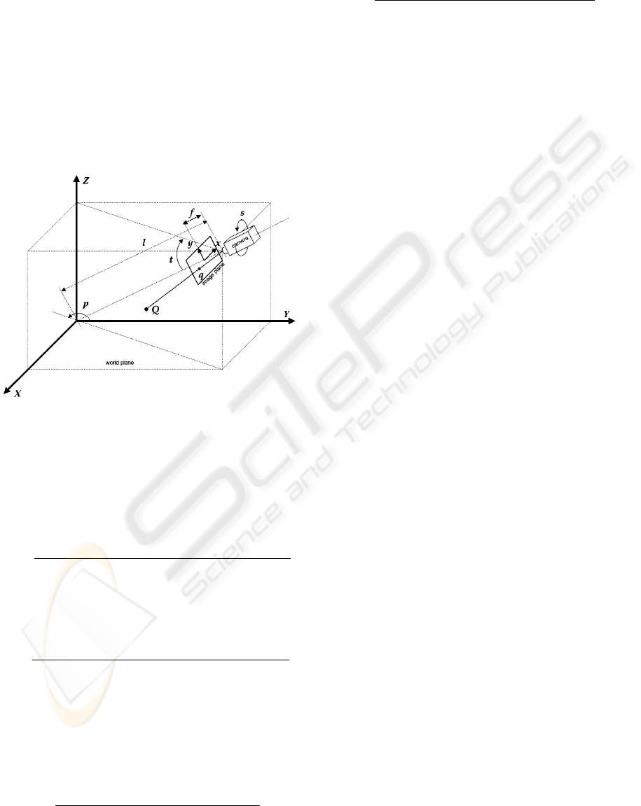
The camera model we use is the one proposed in (He

and Yung, 2007) and (Fung et al., 2003), which is de-

picted in ﬁgure 1. This model describes one intrin-

sic parameter (focal length f ) of the camera and all

its extrinsic parameters (height h, pan angle p, swing

angle s and tilt angle t), and deﬁnes the relationship

between the image coordinates and the world coordi-

nates in terms of these parameters.

Figure 1: Used camera model (He and Yung, 2007).

Let Q = (X

) be an arbitrary point in the

3D world coordinates and q = (x

) be the corre-

sponding 2D image coordinates of Q. The equations

that relate these two points are





(cos p coss + sin p sint sins)

(sin p coss − cos p sint sin s)

cost sins





−X

sin p cost + Y

cos p cost + Z

sint + h/sint

(1)

and





(− cos p sin s + sin p sint cos s)

(− sin p sin s − cos p sint cos s)

cost sins





−X

sin p cost + Y

cos p cost + Z

sint + h/sint

(2)

If we assume that point Q lies on the X-Y plane

then Z

becomes zero and (X

) can be calcu-

lated from (x

) as:



h sin p (x

sins + y

coss) / sint

+ h cos p (x

coss − y

sins)



cost sint + y

cost cos s + f sint

(3)

and



− h cos p (x

sins + y

coss) / sint

+ h sin p (x

coss − y

sins)



cost sint + y

cost cos s + f sint

. (4)

These four equations deﬁne the transformation be-

tween the world coordinates and image coordinates,

knowing the camera parameters. To estimate these

parameters, a calibration pattern of known dimen-

sions is necessary. Next section describes the proce-

dure used to get it.

2.2 Finding a Good Calibration Pattern

The desired calibration pattern is based on the road

lane markings. The ﬁrst thing needed to automatically

ﬁnd such a calibration pattern is a good image of the

road to work with. Typically, the background image

is a good solution.

2.2.1 Background Image

The method used is based on the Σ − ∆ ﬁlter and

belongs to the substraction technique (Manzanera,

2008). Its operating principle is to calculate a tempo-

ral and local activity map, in order to deﬁne automat-

ically the thresholds used to decide if a pixel belongs

to the background or to the foreground, these thresh-

olds being variable spatially and temporally (see ﬁg-

ure 2a).

2.2.2 Lane Markings Detection

Parallel Lines. First of all, the assumption that lane

markings are almost parallel to each other and ap-

proximate straight lines is made.

To detect lane markings, a ﬁlter is applied many times

to the background image, but with different parame-

ter values. This ﬁlter determines pixels whose neigh-

borhood (ﬁrst parameter) is brighter than itself with

a certain tolerance (second parameter). The resulting

images obtained with this ﬁlter will then be processed.

For each image, a label is assigned to each binary con-

nected components and some of their shape proper-

ties are measured (i.e. the surface, eccentricity, ori-

entation and centroid). Once this has been done, the

properties of the obtained groups in each image are

compared. The ones with more or less stable proper-

ties in all the images are kept. Finally, the groups that

do not comply with certain constraints are rejected.

The remaining groups correspond to various objects

considered as possible lane markings (see ﬁgure 2b).

After that, one virtual line is created per detected

object, each line passing through the centroid and

A CAMERA AUTO-CALIBRATION ALGORITHM FOR REALTIME ROAD TRAFFIC ANALYSIS

627

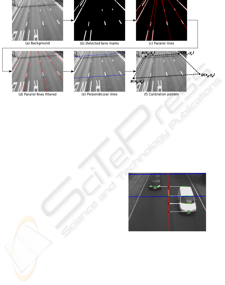
Figure 2: Calibration pattern algorithm.

having the same orientation as its corresponding ob-

ject (ﬁgure 2c). These virtual lines are called parallel

lines.

These parallel lines are ﬁltered to retrieve the ones

corresponding to real lane markings (see ﬁgure 2d).

The ﬁltering process has three steps. The ﬁrst one

consists in merging parallel lines whose centroids and

orientation are fairly close. The second step is based

on the neighborhood of each parallel line. For each

parallel line, the neighborhood in the background im-

age is analysed to ﬁnd bright objects and count them.

Any parallel lines for which too few objects were

found are deleted. Finally, the last step checks the

distance between parallel lines and rejects bad ones.

Once all of this has been done, parallel lines are ob-

tained.

Perpendicular lines. Once the parallel lines have

been detected, ﬁnding perpendicular lines can be done

easily. Pixel brightness along every parallel line is

analysed to ﬁnd the beginnings and ends of lane mark-

ings along that line. Depending on the situation, two

methods can be used to ﬁnd perpendicular lines. The

ﬁrst one works only on roads with at least three lanes

while the second one works on roads with at least two

lanes.

For the ﬁrst method, it is assumed that discontinu-

ous lane markings are more or less synchronous in the

3D space. Starting from this assumption, the parallel

lines detected before are analysed to ﬁnd lane mark-

ings. Then, virtual lines passing through the corre-

sponding lane markings of each parallel line are cre-

ated, as shown in ﬁgure 2e. These virtual lines are

called perpendicular lines.

For a two lanes road, there are only two continuous

lane markings on the edge of the road and one discon-

tinuous lane marking in the middle. A perpendicular

line is obtained by taking a point (called pivot point)

on the parallel line passing through the discontinu-

ous lane marking. The trafﬁc is then analysed to ﬁnd

near perpendicular lines on vehicles with the assump-

tion that they are travelling along road axis. Each

time such a line is detected passing near a pivot point,

its orientation is used to adjust the perpendicular line

passing through that pivot point, as shown in ﬁgure 3.

Figure 3: Perpendicular lines on a two lanes road.

2.2.3 Calibration Pattern

After the lane markings detection, intersections of

parallel and perpendicular lines are calculated and the

four points farthest from each other are kept. These

points form the parallelogram used as calibration pat-

tern to calibrate the camera, as shown in ﬁgure 2f.

The reason why a calibration pattern as large as pos-

sible is desired is that it helps minimize the error due

to poor positioning points.

VISAPP 2009 - International Conference on Computer Vision Theory and Applications

628

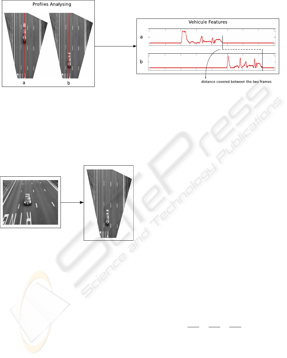
Figure 4: Features extraction from two consecutive frames a and b.

2.3 Camera Calibration

Once a good calibration pattern is found, the camera

parameters are estimated with the method proposed in

(He and Yung, 2007). The equations (3) and (4) are

then used to project the images on the X − Y plane of

the 3D world (Z

= 0), as shown in the ﬁgure 5.

Figure 5: Image projection.

3 VEHICLE FEATURES

EXTRACTION

Extracting vehicle features implies detecting the traf-

ﬁc. A common way to do this is to subtract the

background image (see section 2.2.1) from the current

frame to get a foreground image. In this approach, in-

stead of working with the whole image, virtual lines

called proﬁle are used. Figure 4 shows an example

of one proﬁle analysis. For the sake of clarity, just

one proﬁle is shown in this example but, of course, as

many proﬁles as necessary can be deﬁned. Typically,

ﬁve proﬁles per lane is quite sufﬁcient.

3.1 Speed Estimation

Once features of a vehicle have been extracted from

two frames, estimating its speed by measuring the dis-

tance between the beginning of its signal in successive

frames is possible, as shown in ﬁgure 4.

3.2 Height Estimation

Based on the deformations visible on vehicle proﬁle

(due to the perspective effect), estimating the height

of this vehicle is possible. Indeed, the equations (3)

and (4) used for the transformation from image coor-

dinates to world coordinates project the images on the

X-Y plane of the 3D world. This implies two things.

First, the more a point is high above the ground,

the more its distance from the camera will be over-

estimated. And second, the more a point above the

ground is far away from the camera, the more its dis-

tance from the camera will be over-estimated too. So,

a relation between the height of a vehicle and the de-

formation of his proﬁle from a frame to another can

be found.

Figure 6 shows what happens when a car (repre-

sented here by a box) approaches the camera. Be-

cause the points A and B are known, distance c can be

calculated. Then, through the tilt angle of the camera,

angles

A and

are obtained, wich leads to

and

Finaly, using the classical law of sines

sin

(5)

length a and height h of the vehicule are found.

4 EXPERIMENTAL RESULTS

To validate the features extraction and the speed esti-

mation method, a test was conducted on a video se-

quence. The results are presented in table 1. For your

A CAMERA AUTO-CALIBRATION ALGORITHM FOR REALTIME ROAD TRAFFIC ANALYSIS

629

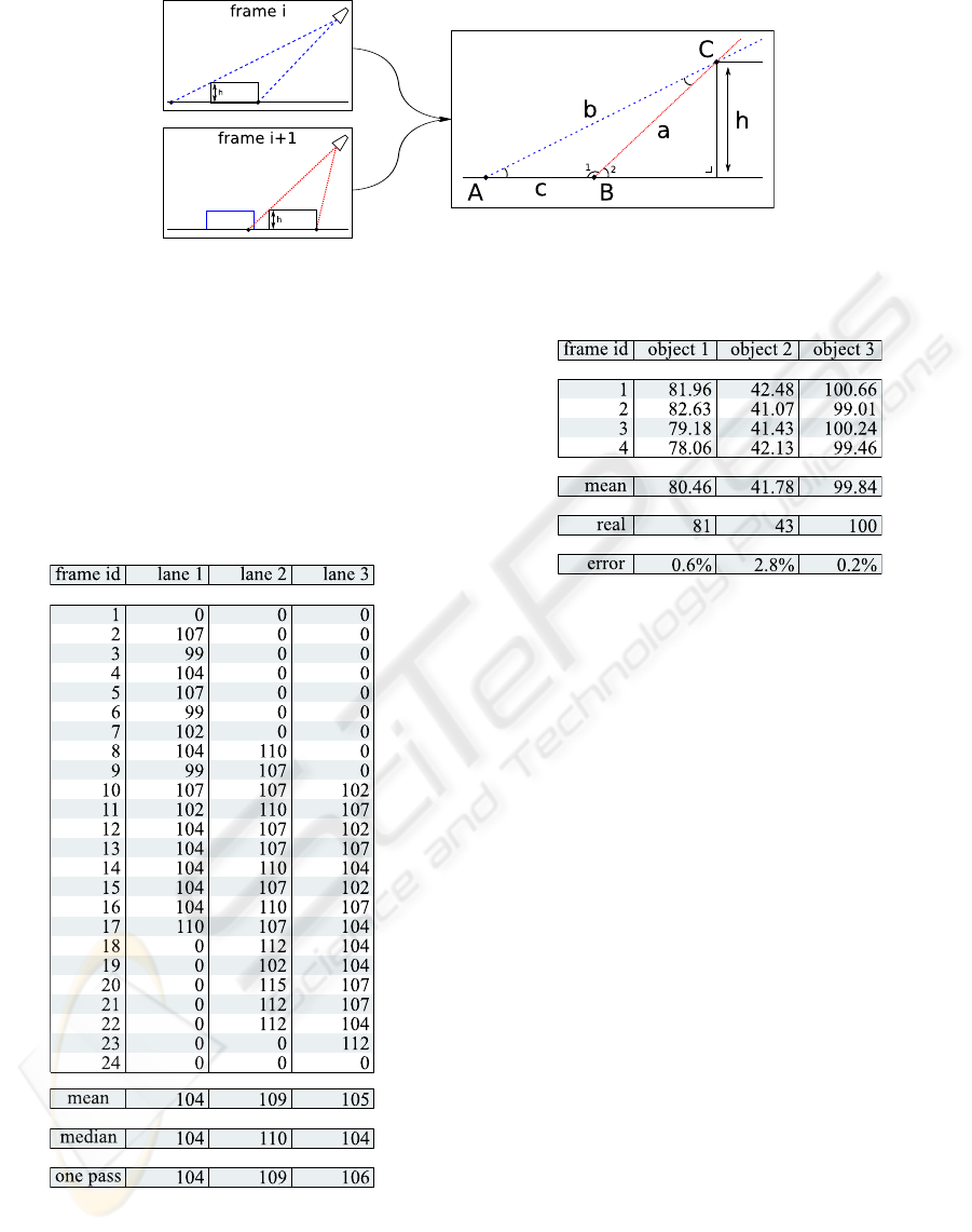
Figure 6: Vehicle height estimation.

information, the last value one pass corresponds to

the estimated speed, using only the ﬁrst and the last

frame (i.e. the ﬁrst frame in which the vehicle is visi-

ble and the last one in which it is still visible). Un-

fortunately, these results could not be validated for

lack of radar measures. However, they ensured us that

the estimated speed was consistent compared with the

video sequence.

Table 1: Estimation speed results (in km/h).

To validate height estimation method, a chess-

board with known dimensions is used to calibrate the

camera. Then, two pictures of moving objects on the

chessboard are taken. Finally, the height of these ob-

jects is estimated. Table 2 shows that results have an

estimation error of less than 3%.

Table 2: Estimation height results (in mm).

5 CONCLUSIONS AND FUTURE

WORK

In conclusion, a mono-camera system for trafﬁc mon-

itoring that can accurately and automatically calibrate

itself has been presented. It detects all the vehicles

and estimates their speed, and because it doesn’t need

all the image pixels to work, it is quite efﬁcient. Addi-

tionally, a method to estimate vehicle height has been

presented which, according to ﬁrst tests, should op-

erate relatively well. Furthermore, once the vehicle

height will be known, estimating its width and length

will be possible.

REFERENCES

Dickinson, K.W., and Wan, C. (1989). Road trafﬁc moni-

toring using the trip ii system. In Second International

Conference on Road Trafﬁc Monitoring.

Fung, G. S. K., Yung, N. H. C., and Pang, G. K. H. (2003).

Camera calibration from road lane markings. Optical

Engineering, 42(10).

He, X. C. and Yung, N. H. C. (2007). New method for

overcoming ill-conditioning in vanishing-point-based

camera calibration. Optical Engineering, 46(3).

Hogg, D. C., Sullivan, G. D., Baker, K. D., and Mott, D. H.

(1984). Recognition of vehicles in trafﬁc scenes using

VISAPP 2009 - International Conference on Computer Vision Theory and Applications

630

geometric models. In Road Trafﬁc Data Collection,

volume 242, pages 115–119.

jun Tan, X., Li, J., and Liu, C. (2007). A video-based

real-time vehicle detection method by classiﬁed back-

ground learning. World Transactions on Engineering

and Technology Education.

Kastrinaki, V., Zervakis, M., and Kalaitzakis, K. (2003). A

survey of video processing techniques for trafﬁc appli-

cations. Image and Vision Computing, 21:359–381.

Manzanera, A. (2008). Progress in Pattern Recognition,

Image Analysis and Applications, volume 4756/2008

of Lecture Notes in Computer Science, chapter Σ − ∆

Background Subtraction and the Zipf Law, pages 42–

51.

A CAMERA AUTO-CALIBRATION ALGORITHM FOR REALTIME ROAD TRAFFIC ANALYSIS

631

REFERENCES

Dickinson, K.W., and Wan, C. (1989). Road traffic moni-