
DEVELOPMENT AND APPLICATION OF A ROACH
GENE REGULATION PROFILE BASED GENDER
DISCRIMINATION METHOD
Yongxiang Fang
Department Mathematics & Statistics, Lancaster University, Lancaster, LA1 4YF, U.K.
Keywords: Data analysis, Microarray study, Gender discrimination, Gene regulation profile.
Abstract: This study extracted, from a roach gonad microarray data set, a gene regulation profile in contrast of male
and female roaches. Then a method is developed to use this profile to discriminate the genders of the
roaches involved in another roach microarray experiments in which the roaches are too young for their
genders to be classifiable. The gender is an ignorable factor in roach gene expression study and the gender
information is vital for the success of such a microarray study, because without the gender information the
treatment effects could not be estimated correctly. A comparison of the analytical results of target data set
based on with and without concerning the gender effects shows that the estimation of treatment effects is
improved greatly when obtained gender information is incorporated in the data analysis. This is reversely
evident that the roach gender discrimination method developed in this study performs very well.
1 INTRODUCTION
Roach is a major species of fish in still and slow
moving waters in Europe. The fish has been adopted
widely for assessing contaminant effects, and most
notably for studies endocrine disrupting chemicals.
This is because roach can develop as either a male or
female (Schultz, 1996) and feminization of male in
the wild can arise through exposing to oestrogen
mimic chemicals (Gibson et al., 2005; Jobling et al.,
2006; Katsu et al., 2007).
A roach microarray study observes the gene
response of roaches to
17a-ethinylestradiol (EE2)
Figure 1: Experimental design of roach 720 days
microarray study.
contaminated water instantly after fertilisation until
they reach different ages which include 84, 250 and
720 days. The 720 days roach gonad microarray
experiment was design to identify the genes that
express differently between male and female gonads
and genes that respond to EE2 treatment. Four
groups of samples are selected for the experiment
and they are: Control male (CM), control female
(CF), exposed male (EM) and exposed female (EF).
The control samples are extracted from roach in EE2
free water. The treatment samples are extracted from
roaches exposed EE2 contaminated water for 720
days. The experiment uses two-colour cDAN
microarray and follows a four-vertex interwoven
loops design. Dye swap technique is employed in the
experiment too, see figure 1. The microarray data is
analysed though data normalization, PCA analysis,
modelling, fitting, testing, differentially expressed
gene extracting, clustering and gene ontology term
based analysis. Data normalization includes VSN
(Variance Stabilization Normalization, Huber et al.,
2002), Lowess (Cleveland, 1979; Cleveland and
Delvin, 1988) for dye bias correction, and 2-D
Lowess for spatial normalization. Principal
Component Analysis (PCA) is applied to normalized
data and the second and third component are plotted
in figure 2. The plot reveals that control male and
control female can be separated clearly, in contrast,
Exposed M
Control M
Control F
Exposed F
263
Fang Y. (2009).
DEVELOPMENT AND APPLICATION OF A ROACH GENE REGULATION PROFILE BASED GENDER DISCRIMINATION METHOD.
In Proceedings of the International Conference on Knowledge Discovery and Information Retrieval, pages 263-269
DOI: 10.5220/0002275302630269
Copyright
c
SciTePress
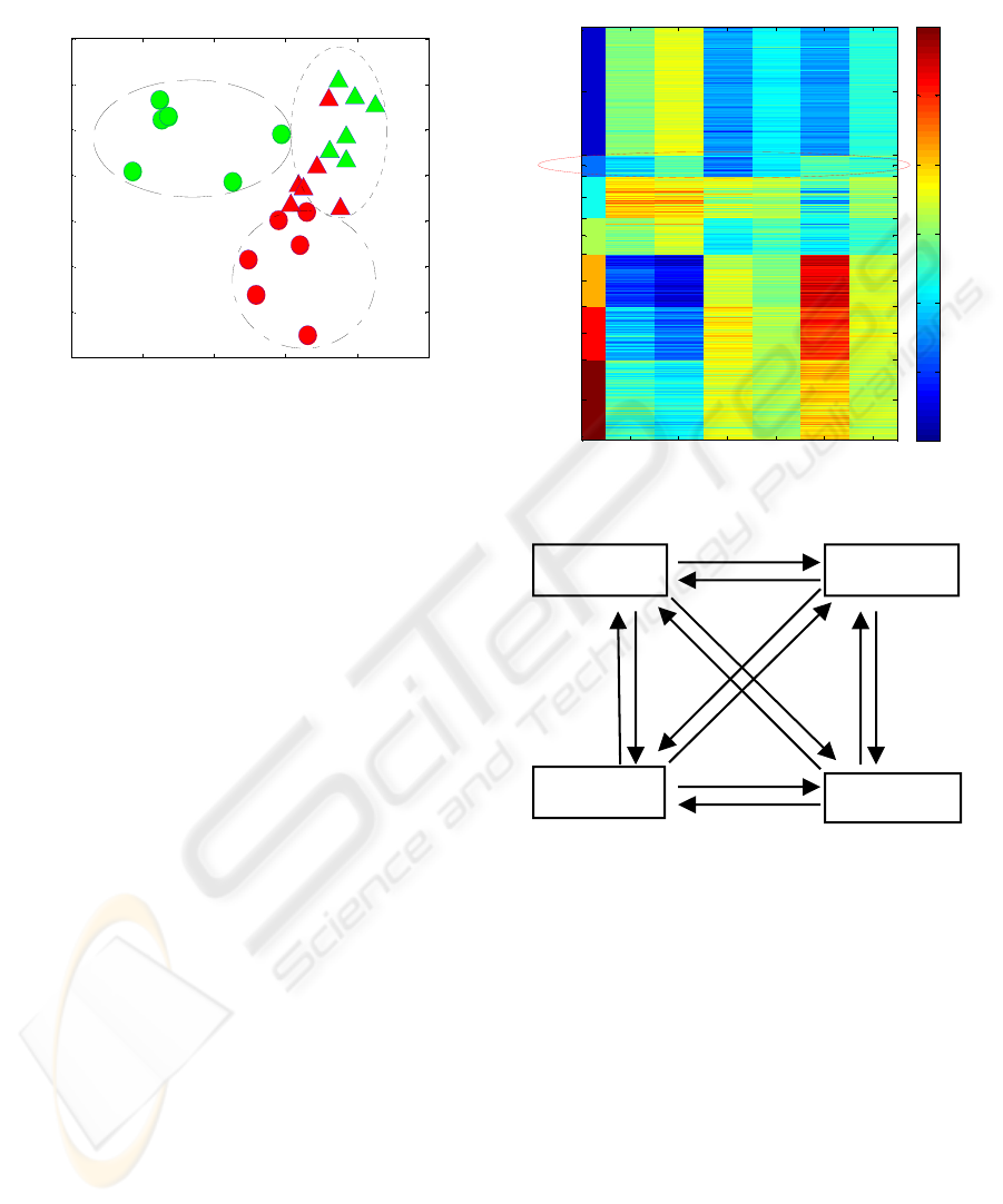
exposed male and exposed female tend to be similar.
The figure 2 also shows that male responds stronger
and becomes female like.
Figure 2: PCA plot of the roach 720 days dataset.
The further analysis employs a linear model to
model the normalized data (Wit and Khanin, 2005)
and the LS (Least Squares) approach to achieve
maximum likelihood estimation. The estimated log-
ratio values are tested by t-test and then the
differentially expressed (DE) genes are identified by
FDR control (Benjamini and Hochberg, 1995, 2000)
at 5% level. The DE genes are clustered and the
results are visualized by a heat-map (Figure 3).
Where the log-ratio values are visualised by colours
based on the scale of the colour bar; the columns
present parameters corresponding different
comparisons of sample groups; the rows resent DE
genes which are clustered into 7 clusters.
The experimental design of the 84 days roach
microarray study is illustrated in figure 4, which has
also four sample groups: controls (C), exposure
level-1 (E1, 0.1 ng/L), level-2 (E2, 1ng/L) and level-
3 (E3, 10 ng/L) treatments. This study has two
differences from 720 days roach study. Firstly, the
mRNA is extracted from the whole body of sample
roaches. Secondly, the roaches of 84 days old are too
young to be gender classifiable, i.e. the sample’s
gender is unknown. The measured data is analysed
the same way as applied to the 720 days data set,
however, the gender effects are not able to be
incorporated into data model. Figure 5 is the
histogram of p-values from testing the estimated
parameter values (log
2
-ratios). It clearly shows that
all the three subplots for comparisons E1 vs C, E2 vs
C and E3 vs C are almost flat, i.e. there is hardly any
presence of DE genes. Concordantly, no gene is
identified as DE gene by controlling FDR at level as
high as 20%. This suggests that under the settings of
84 days experiment, EE2 contaminated water do not
have notable genetic impact on roaches.
Figure 3: Heat-map of clusters of DE genes for the roach
720 days data set.
Figure 4: Experimental design of the 84 days roach
microarray study.
The results from the 720 days data set and the 84
days data set lead to obviously different pictures of
the effects of similar treatments, and most likely
only one of them is correct. Owing to the 720 days
data set is concordant with the facts observed by
environment and fish biological studies while the
result of the 84 days data set is from a model without
considering gender effects, the results from the 84
days data set are less convincing. However, the only
way to make the results of 84 days data set to be
convincing enough is to make sample’s gender
information available and then incorporate gender
effects into data model. Therefore, in order to draw
results correctly from 84 days data set, it is critical to
develop a method by which the gender of young
roaches can be discriminated correctly.
-0.15 -0.1 -0.05 0 0.05 0.1
-0.08
-0.06
-0.04
-0.02
0
0.02
0.04
0.06
Com
p
onent 2
Component 3
Control
Female
Exposed
Control
Male
Significant probes
cluster CM/CF CM/EF EM/CF EM/EF EM/CM EF/CF
C1
1464
C2
1702
C3
2177
C4
2593
C5
3182
C6
3788
C7
4705
-6
-4
-2
0
2
4
6
Control
E3
E2
E1
KDIR 2009 - International Conference on Knowledge Discovery and Information Retrieval
264

Figure 5: Experimental design of the 84 days roach.
This gender discrimination is very challenging
and very significance as well. Because by properly
identifying and selecting such genes, a gender gene
regulation profile can be developed and used to
recognize the gender of sample roaches in the 84
days experiment. Hence, we can incorporate gender
effects into data model and estimate both the
treatment effects and gender effects simultaneously.
We can expect to get better results, if and only if the
genders of sample roaches are identified correctly.
This means that the new results of the 84 days data
set will be reversely evident of the correctness and
performance of gene regulation profile extracted
from the 720 days data set.
2 METHOD
2.1 Development of a Roach Gene
Regulation Profile for Gender
Discrimination
The most critical point in developing a gene
regulation profile for gender discrimination here is
what genes should be selected. In order to have good
and consistent performance in gender
discrimination, we require such genes whose
directions (up or down) of regulation keep
unchanged when the samples of two genders are
compared. Explicitly, the genes are always up-
regulated or down-regulated in comparisons of
different gender including CM vs CF, CM vs EF,
EM vs CF and EM vs EF. In addition, the genes also
should be not obviously regulated in the
comparisons of same gender including EM vs CM
and EF vs CF. In fact, the regulation of such genes
are dominated by genders and the treatment effects
are subordinate. From heat-map (figure 3), it is easy
to see that genes in all 7 cluster, but cluster 2, are
definitely not suitable to be selected. The genes in
cluster 2 are strongly down regulated in all contrasts
of male sample against female sample. However,
only those genes that are not differently expressed in
contrast of samples of same gender can be selected.
Figure 6 is the heat-map of a further clustering of
cluster 2 based on six comparisons. The heat-map
shows that the cluster 1 contains the best candidate
genes. 20 genes from this cluster are selected and list
in Table 1 to form a gene regulation profile for roach
gender discrimination.
Figure 6: Heat-map of sub-clusters of cluster 2 in figure 3.
Table 1: Selected genes for gene regulation profile of
Male v.s. Female.
GeneID: the identifier of probes on the roach microarray
0 0.5 1
0
1000
2000
3000
Frequency
dye
0 0.5 1
0
1000
2000
3000
E1/C
0 0.5 1
0
1000
2000
3000
E2/C
0 0.5 1
0
1000
2000
3000
P-value
E3/C
Cluster 2
Sub-cls CM/CF CM/EF EM/CF EM/EF EM/CM EF/CF
20
40
60
80
100
120
140
160
180
200
220
-6
-4
-2
0
2
4
6
GeneID CM/CF CM/EF EM/CF EM/EF EM/CM EF/CF
51k23 ‐1.4896 ‐1.6038 ‐2.9792 ‐1.1772 ‐0.0735 0.1142
50j09 ‐1.7335 ‐1.5019 ‐3.4669 ‐0.9522 0.0497 ‐0.2316
53n 01 ‐1.4666 ‐1.3786 ‐2.9332 ‐1.0865 ‐0.2079 ‐0.0880
16g10 ‐2.2736 ‐1.7174 ‐4.5473 ‐2.0497 ‐0.8324 ‐0.5563
16j14 ‐2.1447 ‐1.6470 ‐4.2894 ‐2.0234 ‐0.8765 ‐0.4978
27l14 ‐1.6972 ‐1.4120 ‐3.3945 ‐2.0013 ‐1.0893 ‐0.2852
33f08 ‐1.7677 ‐2.0387 ‐3.5353 ‐0.9249 0.6138 0.2710
34e01 ‐2.2340 ‐2.1768 ‐4.4680 ‐0.7230 0.9538 ‐0.0572
36i24 ‐1.6115 ‐1.7116 ‐
3.2230 ‐1.2338 ‐0.0222 0.1001
36k18 ‐2.0110 ‐1.4390 ‐4.0221 ‐1.5069 ‐0.5678 ‐0.5720
40f22 ‐2.0219 ‐1.4596 ‐4.0438 ‐1.6408 ‐0.6812 ‐0.5623
48i19 ‐1.9387 ‐1.4107 ‐3.8773 ‐1.6595 ‐0.7488 ‐0.5279
03j21 ‐1.9768 ‐1.4795 ‐3.9535 ‐1.7592 ‐0.7797 ‐0.4973
52b 21 ‐1.9373 ‐1.3759 ‐3.8745 ‐1.5978 ‐0.7218 ‐0.5613
52e23 ‐2.1635 ‐0.9611 ‐4.3270 ‐0.9602 0.0009 ‐1.2024
52i03 ‐2.1172 ‐1.8005 ‐4.2344 ‐2.3163 ‐1.0158 ‐0.3167
53e19 ‐1.9954 ‐1.5432 ‐3.9909
‐1.7039 ‐0.6606 ‐0.4522
55g11 ‐2.0688 ‐1.5076 ‐4.1375 ‐1.3684 ‐0.3608 ‐0.5612
62f20 ‐1.6039 ‐1.7681 ‐3.2078 ‐1.0665 0.2016 0.1643
63h 03 ‐1.7090 ‐1.4808 ‐3.4179 ‐0.6749 0.3059 ‐0.2282
DEVELOPMENT AND APPLICATION OF A ROACH GENE REGULATION PROFILE BASED GENDER
DISCRIMINATION METHOD
265

2.2 The Gender Regulation Profile
of Two Samples on a Roach
Microarray
Table 1 lists the genes which are selected to
represent the regulation profile between male and
female roach. Based on this, a gene regulation
profile reflecting the sample’s genders on a
microarray can be described by the measured log-
ratios at these gene spots. Therefore, for given a
roach microarray, the log-ratio values on
corresponding probes provide the information about
the genders of the roaches measured on this array.
2.3 Test Statistic and Test Method
Up to now, we have a gene regulation profile for
male vs female; we also can extract a gene
regulation profile for roaches measured on a
microarray. The task now is how to judge the
samples’ genders based on the two profiles. For
simplicity, the gene regulation profile built on the
720 days data will be referred as the reference
profile and the gene regulation profile extracted
from a target microarray will be called a query
profile.
Two statistical test methods are proposed and
applied. The first method is sign test which takes the
number of data points of same sign in a query profile
as test statistic. A positive value in a query profile
means this gene is up-regulated in cy5 sample
against cy3 sample; and the opposite is true for a
negative value. There are 20 genes in a profile, i.e.
20 log-ratio values, if two samples measured on a
microarray have same sex, the number of the data
points with positive (‘+’) sign and that with negative
sign (‘-‘) in the query profile are expected to be
equal. This can be taken as the null case and the
corresponding null distribution is formulated by a
binomial distribution function: b(20,0.5). Now to
take the number of negative signs in a query profile
as the test statistic, then if this statistic significantly
differs from 10, the profile can be judged to be
similar or opposite to reference profile. This can be
easily achieved by one side test of the statistic based
on b(20,0.5). If the profile is tested similar to
reference profile, then assigns male as the gender for
cy5 sample and female as the gender of cy3 sample,
vice versa. If the test is not significant in both sides,
the genders of cy3 sample and cy5 sample are same,
though we do not know that they are either male or
female.
The second method employs t-test of the
concordance between reference profile and query
profile. The concordance coefficient is defined to be
similar but not the same as Pearson’s Correlation
Coefficient. Denoting by P
r
and P
q
the reference
profile and query profile respectively and C(P
r
,P
q
)
the concordance coefficient of the two profiles is
formulated as:
,
(1)
Based on formula (1), the major difference
between concordance coefficient and Pearson’s
correlation coefficient is that: the mean of P
r
and
mean of P
q
impact on the value of concordance
coefficient, but they will to do nothing with the
value of Pearson’s correlation coefficient, because,
in the computation of Pearson’s correlation
coefficient, they are simply removed. Therefore, the
only case which allows the concordance coefficient
and Pearson’s correlation coefficient to have the
same value is that P
r
and P
q
have zero mean.
The use of the concordance instead of correlation
to assess the relationship between two gene
regulation profiles is vitally important, and for
obvious reasons. Because a value in a profile reflects
how a gene is regulated in contrast of cy5 sample
against cy3 sample: positive value for up-regulation
while negative value for down regulation. When
two profiles P
r
and P
q
are assessed, it should
guarantee a element to have positive contribution
when the element has the same sign in P
r
and P
q
, and
the opposite is true when the element has different
sign in P
r
and P
q
. This demand is satisfied in using
concordance coefficient. However, this might not
retain in the case when Pearson’s correlation
coefficient is used. For example, if the vector mean
for both P
r
and P
q
is 2, and the dispersion within
profiles are normal noises of small values, that is
2
,
|
|
1 and
2
,
1.
Due to each gene in query profile is about equally
regulated as corresponding gene in reference profile,
the two gene regulation profiles should be judged as
closely the same. However, Pearson’s correlation
coefficient of the two profiles will be around 0,
because
,
,
in this case. The
judgement based on Pearson’s correlation coefficient
will consequently be: the two profiles are nothing in
common, which is wrong and definitely
unreasonable. In contrast, from formula (1) the
concordance coefficient of the two profiles will be
,
1. Consequently, to conclude that the
two profiles are almost identical is reasonable and
correct.
KDIR 2009 - International Conference on Knowledge Discovery and Information Retrieval
266

The concordance coefficient formulated by
similar analogy of correlation coefficient allows us
to borrow some properties of correlation coefficient
and the technique to transfer it into a t statistic.
Obviously, the concordance coefficient will be
valued as real number in the interval [-1,1]. The
value 1 means two vectors are exactly the same; the
value -1 implies that the two vectors are only
different by a negative sign. While the value zero
presents that the two vectors are orthogonal.
Pearson’s correlation coefficient can be transferred
into a t statistic by (2) below, where, n is length of
the vector from which the correlation coefficient is
computed, and t
n-2
is t statistic with n-2 degree of
freedom:
(2)
Therefore, the significance of Pearson’s
correlation coefficient can be tested by t-test. For
concordance coefficient, such approach can be
applied in the similar way.
In fact, let
,
and let
,
, then we have:
,
,
,
(3)
Where
,
is Pearson’s correlation
coefficient of P
1
and P
2
; and
,
can be
transferred into a t statistic with n-1 degree of
freedom and n is the length of the vector P
r
.
In summary, the concordance of reference
profile and query profile is measured by equation
(1), the significance of this measurement can be
transferred into t statistic by:
(4)
For given significance level α and the length of
the vector n, the critical value of concordance
coefficient can be shown as:
,
,
1
,
(5)
If take the significance level 0.05 and
replace n with 20 - the number of genes in our gene
regulation profile, the critical values of concordance
coefficient are 0.3687. For our practical case, if
query profile of a microarray from the 84 day
experiment have a concordance coefficient greater
than 0.3687, the cy5 sample is male and cy3 sample
is female. In contrast, if the concordance coefficient
is less than -0.3687, the cy5 sample is female and
cy3 sample is male. Otherwise, the samples on two
channels have the same gender.
3 APPLICATION
3.1 Reference Profile
and Query Profiles
The genes in reference profile are listed in table 1,
and the row mean of the first four columns is the
reference profile P
r
. For each array in the 84 days
roach data set, a query profile is formed by log-ratio
values shown by this array at the probes listed in
table 1.
3.2 Statistic and Hypotheses
For sign test, the statistic is the count of negative
sign in query profile. The null hypothesis is H
0
: the
number of the ‘+’ and ‘-‘ are same, the alternative
hypothesis is: H
1
: the number of the ‘-‘ is more
(less) than ‘+’.
For concordance based test, the statistic t-
statistic formulated by equation (4), where the
concordance coefficient C is defined by equation
(1). The hypotheses of the test are H
0
: c = 0 vs H
1
:
c>0 (c<0). Let significance level be 0.05, the critical
values of the test are 0.3687.
3.3 Results of Test
The values of sign statistic and t statistic for 12
microarrays in 84 days roach experiment are list in
table 2. The p-values of the tests and the gender
assigned to each sample are listed there too. Table 2
shows the gender discrimination based on the results
from sign test and t-test are same in our case.
Table 2: Identified gender of sample roaches in 84 days
experiment.
Array No
statistic
s (sign) P(S<=s) P(S>=s)
statistic
t
P( T < =t )
P( T > =t )
Cy 5
sample
gender
Cy 3
sample
gender
1 3 0.0013 0.9998 ‐4.996 0 1
FM
20 01‐14.89 0 1
FM
3 18 1 0.0002 5.098 1 0
MF
40 01‐10.45 0 1
FM
50 01‐9.196 0 1
FM
6 11 0.7483 0.4119 ‐0.844 0.2049 0.795
M (F)
M(F )
7 20 1 0 7.3138 1 0
MF
8 17 0.9998 0.0013 4.5308 0.9999 1E‐04
MF
9 20 1 0 8.9722 1 0
MF
10 20 1 0 11.701 1 0
MF
11 4 0.0059 0.9987 ‐3.55 0.0011 0.999
FM
12 2 0.0002 1 ‐5.777 0 1
FM
DEVELOPMENT AND APPLICATION OF A ROACH GENE REGULATION PROFILE BASED GENDER
DISCRIMINATION METHOD
267
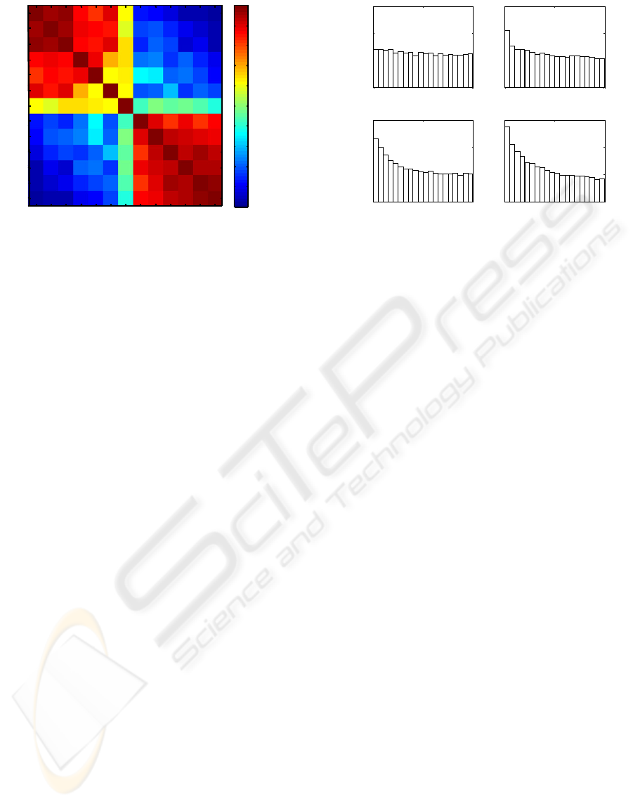
Figure 7: Visualization of the concordance of profiles. All
F/M microarrays are positioned to left hand side and M/F
microarrays are positioned to right hand side. Profiles
within F/M are concordant positively. It is the same for
profiles within M/F. However, profiles between F/M and
M/F profiles are negatively concordant.
The concordance coefficients between reference
profile and query profiles of 12 arrays are illustrated
in Figure 7. The orders of 12 query profiles are
rearranged based on discriminated gender. It shows
that the profiles are strong positively concordant
within F/M or F/M block, while the profiles are
strong negatively concordant between F/M and M/F
blocks. However, array 6 is not significantly
concordant with either F/M block or M/F block,
hence the gender of the two samples measured on
the array are same in gender.
3.4 The Results from Model with and
Without Gender Factor
Before the gender of the samples in the 84 days data
set is discriminated, the linear model for the data set
cannot consider the effects of gender. The effects of
EE2 treatment are estimated by ignoring the gender
effects. The histogram of p-values of fitted
parameters for treatment effects is shown in figure 5,
which indicts that the EE2 treatment seems without
any significant effects on gene expression. This is
not concordant with either the results from the 720
days data set or relevant fish biology studies.
When the samples are labelled by the
discriminated gender and gender effects are included
into the model, both treatment effects and gender
effects can be estimated and tested based the new
model.
Figure 8 shows the histogram of p-values of the
estimations. Based on the p-value distributions, it is
Figure 8: Histogram of P-values from model with both
treatment and gender effects.
estimated to have a thousands of probes are
significantly differently expressed and 581 DE
probes are extracted by control the level of FDR at
20%. This is very different from the results output
from data model without considering gender effects.
In addition, it reveals that the treatment effects
increase as the concentration level of EE2 goes up.
The level-1 treatment hardly shows any significant
genes, the effects of level-2 and level-3 treatments
obviously stand out. However, the number of genes
being impacted by level-2 treatment is considerable
less the number of genes being affected by level-3
treatment. This outcome is concordant with opinion
of biologist other relevant studies.
4 FUTURE WORK
This study developed a gene regulated based gender
profile and used it for discriminating the genders of
young roaches which are not gender classifiable by
other available ways. The application of proposed
approach to practical data confirmed that the method
has good performance. Actually, this method is
potential useful in broader area, such as inspection
and control the impacts of EE2 pollution. The idea
of one future work is to catches the wild roach from
inspected environment, discriminate their genders by
this approach; then focus on the male roaches and
examine they respect to feminization; the degree of
feminization of male roach is a convincing index of
biological impacts of EE2 contamination to the
environment.
The second effort in the future is to improve the
gene regulation profile used in this study, because
the current profile is based on majorly unknown
Array Number
2 4 5 12 1 11 6 8 3 7 9 10 ref
2
4
5
12
1
11
6
8
3
7
9
10
ref
-1
-0.8
-0.6
-0.4
-0.2
0
0.2
0.4
0.6
0.8
1
0 0.5 1
0
1000
2000
3000
E1/C
0 0.5 1
0
1000
2000
3000
E2/C
0 0.5 1
0
1000
2000
3000
Frequency
E3/C
0 0.5 1
0
1000
2000
3000
P-value
F/M
KDIR 2009 - International Conference on Knowledge Discovery and Information Retrieval
268

sequences. The improvement will replace the
unknown sequences in the profile with annotated
fish genes which may be identified to be suitable for
roach gender discrimination.
ACKNOWLEDGEMENTS
This work was supported by NERC grants NE/
F001355/1.
REFERENCES
Benjamini, Y. and Hochberg, Y., 1995. Controlling the
false discovery rate: A practical and powerful
approach to multiple testing. J. Roy. Statist. Soc. Ser.
B 57 289--300.
Benjamini, Y. and Hochberg, Y., 2000. On the adaptive
control of the false discovery rate in multiple testing
with independent statistics. J. Educational and
Behavioral Statistics 25 60--83.
Cleveland, W.S. and Delvin, S.J., 1988. Locally weighted
regression: An approach to regression analysis by
local fitting. Journal of American Statistical
Association, Vol. 83, pp. 596-610.
Cleveland, W.S., 1979. Robust locally weighted
regression and smoothing scatterplots. Journal of
American Statistical Association, Vol. 74, pp. 829-
836.
Gibson, R., Smith, M. D., Spary, C. J., Tyler, C. R., and
Hill, E. M., 2005. Mixtures of estrogenic contaminants
in bile of fish exposed to wastewater treatment works
effluents. Environmental Science & Technology 39,
2461-2471.
Huber, W., von Heydebreck, A., Sultmann, H., Poustka,
A., Vingron, M., 2002. Variance stabilization applied
to microarray data calibration and to the quantification
of differential expression. Bioinformatics 18 (Suppl.
1), S96-S104.
Jobling, S., Williams, R., Johnson, A., Taylor, A., Gross-
Sorokin, M., Nolan, M., Tyler, C. R., van Aerle, R.,
Santos, E., and Brighty, G., 2006. Predicted exposures
to steroid estrogens in U.K. rivers correlate with
widespread sexual disruption in wild fish populations.
Environmental Health Perspectives 114, 32–39.
Katsu, Y., Lange, A., Urushitani, H., Ichikawa, R., Paull,
G. C., Cahill, L. L., Jobling, S., Tyler, C. R., and
Iguchi, T., 2007. Functional associations between two
estrogen receptors, environmental estrogens, and
sexual disruption in the roach (Rutilus rutilus).
Environmental Science & Technology 41, 3368-3374.
Schultz, H., 1996. Drastic decline of the proportion of
males in the roach (Rutilus rutilus L.) population of
Bautzen reservoir (Saxony, Germany): result of direct
and indirect effects of biomanipulation. Limnologica
26, 153–164.
Wit, E., Nobile, A., and Khanin, R., 2005. Near-optimal
designs for dual-channel microarray studies. Applied
Statistics 54, 817-830.
DEVELOPMENT AND APPLICATION OF A ROACH GENE REGULATION PROFILE BASED GENDER
DISCRIMINATION METHOD
269
