DYNAMIC AND EVOLUTIONARY MULTI-OBJECTIVE
OPTIMIZATION FOR SENSOR SELECTION IN SENSOR
NETWORKS FOR TARGET TRACKING
Nikhil Padhye
Department of Mechanical Engineering, Indian Institute of Technology Kanpur, India
Long Zuo, Chilukuri K. Mohan, Pramod K. Varshney
Dept. of Electrical Engineering and Computer Science, Syracuse University, U.S.A.
Keywords:
Genetic algorithms, Multi-objective optimization, PCRLB, Sensor networks, Target tracking.
Abstract:
When large sensor networks are applied to the task of target tracking, it is necessary to successively identify
subsets of sensors that are most useful at each time instant. Such a task involves simultaneously maximiz-
ing target detection accuracy and minimizing querying cost, addressed in this paper by the application of
multi-objective evolutionary algorithms (MOEAs). NSGA-II, a well-known MOEA, is demonstrated to be
successful in obtaining diverse solutions (trade-off points), when compared to a ”weighted sum” approach that
combines both objectives into a single cost function. We also explore an improvement, LS-DNSGA, which in-
corporates periodic local search into the algorithm, and outperforms standard NSGA-II on the sensor selection
problem.
1 INTRODUCTION
When a large sensor network is used for target track-
ing, it is not practical to constantly query all sensors,
due to practical constraints on computation, sensing
range, communication bandwidth, and energy con-
sumption. The number of sensors to be queried (for
high tracking accuracy) may itself vary, and querying
strategies are desirable that allow the data to deter-
mine which sensors should be queried at successive
instants. This paper addresses the task of successively
identifying subsets of sensors while simultaneously
addressing two conflicting objectives: cost and track-
ing accuracy.
To illustrate our approach, we use a simple formu-
lation of communication cost, which increases with
the number of sensors and the communication dis-
tance (from a sensor to the decision-maker’s loca-
tion). Maximizing (predicted) tracking accuracy is
considered equivalent to minimizing mean squared
error (MSE), and addressed in our approach by
minimizing the Posterior Cramer-Rao Lower Bound
(PCRLB) which provides a theoretical performance
limit of any estimator for a nonlinear filtering prob-
lem. In earlier work (Zuo et al., 2006), we have been
successful in using the posterior CRLB for sensor se-
lection in tracking problems.
A straightforward approach often adopted in the
engineering literature is to attempt to optimize a lin-
ear combination of different objective functions. Ex-
ploring different linear combinations yields solutions
corresponding to different tradeoff points. How-
ever, this approach has serious deficiencies, and is
outperformed by multi-objective evolutionary algo-
rithms (MOEAs) that simultaneously evolve multi-
ple candidate solutions, as discussed in (Deb, 2001),
where the Non-dominated Sorting Genetic Algorithm-
II (NSGA-II) is proposed; other MOEA variations
include SPEA2, PAES and EMOCA (Rajagopalan
et al., 2005). In this paper, we have successfully ap-
plied an improvement of NSGA-II that incorporates
local search.
2 MODELS AND OBJECTIVES
This section describes the target motion model, sensor
model, and the two objectives to be optimized.
160
Padhye N., Zuo L., K. Mohan C. and K. Varshney P. (2009).
DYNAMIC AND EVOLUTIONARY MULTI-OBJECTIVE OPTIMIZATION FOR SENSOR SELECTION IN SENSOR NETWORKS FOR TARGET
TRACKING.
In Proceedings of the International Joint Conference on Computational Intelligence, pages 160-167
DOI: 10.5220/0002324901600167
Copyright
c
 SciTePress

2.1 Target Motion Model
Each target is assumed to be moving in a 2-D Carte-
sian coordinate plane according to a dynamic white
noise acceleration model (Bar-Shalom et al., 2001):
x
k
= Fx
k−1
+ v
k
(1)
where constant F models the state kinematics, and
x
k
= [x
k
˙x
k
y
k
˙y
k
]
T
defines the target state at time k.
Here, x
k
and y
k
denote the target position and, ˙x
k
and
˙y
k
denote the target velocities. v
k
is a white Gaussian
noise with covariance matrix Q.
2.2 Sensor Measurement Model
We assume that homogeneous bearing only sensors
are randomly deployed in a 2D Cartesian coordinate
plane. The fusion center has knowledge about indi-
vidual sensors (e.g., positions and measurement ac-
curacy). When queried, a sensor communicates its
estimate of the target state to the fusion center. The
measurement model is given by:
θ
j
k
= h(x
k
) +w
j
k
= tan
−1

y
k
− y
s
j
x
k
− x
s
j

+ w
j
k
(2)
where θ
j
k
is the original measurement from sensor j
with additive white Gaussian noise w
j
k
, whose vari-
ance is parameterized as R.
2.3 Objectives
Communication cost is computed as follows:
Cost =
n
∑
i=1
(C
0
+C
1
q
(X
ch
− X
i
2
) +(Y
ch
−Y
i
2
)) (3)
Here, (X
ch
, Y
ch
) and (X
i
,Y
i
) denote the coordinates of
cluster head and i
th
queried sensor, respectively. Cost
increases with the number of queried sensors.
Tracking accuracy is estimated using PCRLB on
the estimation error of the target position, summing
up the position bound along each axis at time k+1:
C
k+1
= J
−1
k+1
(1, 1) + J
−1
k+1
(3, 3) (4)
where J
−1
k+1
(1, 1) and J
−1
k+1
(3, 3) are bounds on the
MSE corresponding to x
k+1
and y
k+1
respectively.
Particle filters are used to calculate PCRLB as well
as to estimate the target state. We use the recursive
approach in (Tichavsky et al., 1998) to calculate J
k
,
i.e., sequential FIM, as follows:
J
k+1
= D
22
k
− D
21
k
(J
k
+ D
11
k
)
−1
D
12
k
(5)
where
D
11
k
= E{−∆
x
k
x
k
logp(x
k+1
|x
k
)} (6)
D
12
k
= E{−∆
x
k+1
x
k
logp(x
k+1
|x
k
)} (7)
D
21
k
= E{−∆
x
k
x
k+1
logp(x
k+1
|x
k
)} = (D
12
k
)
T
(8)
D
22
k
= E{−∆
x
k+1
x
k+1
logp(x
k+1
|x
k
)} +
E{−∆
x
k+1
x
k+1
logp(z
k+1
|x
k+1
)} (9)
3 MULTI-OBJECTIVE
OPTIMIZATION
A vector x
1
dominates x
2
if x
1
is not worse than x
2
in
any objective, and x
1
is strictly better than x
2
in some
objective. A decision vector x
1
is Pareto-optimal if
no vector x
2
dominates x
1
. MOO problems require
algorithms that find a well distributed set of Pareto-
optimal solutions with least computational expense.
The ”Weighted Sum” (Wtd.) approach in ad-
dressing MOO problems optimizes a weighted sum of
the individual objective functions, obtaining different
tradeoff solutions by using different weights; unfor-
tunately, this approach has well-known failings (Deb,
2001). In its application to the problem of interest in
this paper, we attempt to minimize F = (w)Cost + (1-
w)PCRLB, for different values of w, first by restrict-
ing the number of sensors chosen (in each step) to 2,
and later allowing this number to vary.
MOEAs provide great promise since they can
simultaneously evolve multiple solutions exploring
regions of the Pareto set. Currently, the most widely
used MOEA is NSGA-II (Deb, 2001), which we have
applied to the sensor selection problem using PCRLB
and communication cost as the two objectives to be
minimized. We have also formulated a new variant,
”Local Search based Dynamic NSGA-II” (LS-
DNSGA), described in Table 1, which has provided
better results on the problem under consideration.
The newly introduced features of LS-DNSGA are:
(1) Population Seeding. At each time step (ex-
cept the first), the initial population is seeded with
80% of the final non-dominated solutions obtained at
the end of previous time step. This mechanism helps
since target positions generally do not vary much in
consecutive time steps.
(2) Local Search. An iterative improvement
procedure is applied periodically to solutions from
the best non-dominated solution front, minimizing F
= wCost + (1− w)PCRLB with
w=
(MaxCost−Cost)
(MaxCost−MinCost)
(MaxCost−Cost)
(MaxCost−MinCost)
+
(MaxPCRLB−PCRLB)
(MaxPCRLB−MinPCRLB)
where, MinCost, MaxCost and MinPCRLB, Max-
PCRLB represent minimum and maximum Cost and
DYNAMIC AND EVOLUTIONARY MULTI-OBJECTIVE OPTIMIZATION FOR SENSOR SELECTION IN SENSOR
NETWORKS FOR TARGET TRACKING
161

PCRLB values in the entire population. Local search
is carried out by repeated successive mutation for
each bit in the candidate solution, accepting the mu-
tation if and only if it decreases F.
Table 1: LS-DNSGA(Local Search based Dynamic Non-
dominated Sorting Genetic Algorithm), executed at each
time step when sensors are to be selected.
Input: Sensor Network Information and
Solutions for time ’t-1 ’
Output: Non-Dominated Sets S
t
for given time ’t’
PopulationSeeding(P
0
)
Evaluation (P
0
)
S
t
:= { }
For gen = 1 to MaxGen
(a) Child Population, Q
gen−1
=
Mutation(Crossover(Selection (P
gen−1
)))
(b) Combined Population, R
gen
=
Merge (P
gen
, Q
gen
)
(c) Non-dominated sorting (R
gen
)
(d) P
gen−1
=
Crowding distance sorting (R
gen
)
(e) Local Search (P
gen−1
), after every τ iterations.
(f) S
t
=
RankOneNonDominatedSolutions (P
gen−1
)
End
4 SIMULATION RESULTS
Several series of simulations were carried out to eval-
uate the proposed algorithm. The first set, discussed
in subsection 4.1, compares LS-DNSGA with a
weighted summation approach, a single objective ap-
proach, and with NSGA-II. The single objective ap-
proach is applied in two ways: a) Exhaustive search
approach searching only sensor subsets of size 2. b)
Single objective GA capable of finding any number of
sensor subsets. In subsection 4.2 LS-DNSGA is ap-
plied and two sensor selection schemes namely, fixed
number of sensors (2) and fixed cost strategy, are in-
vestigated. Finally, subsection 4.3 compares LS-
DNSGA and NSGA-II on larger sensor networks.
The appendix contains details of various parameters
involved in system models, sensor selection schemes
and cost computation.
4.1 Experiment I
In these simulations, we compare the LS-
DNSGA with a single objective approach and
standard NSGA-II. We consider the target tracking
problem, with total number of sensors 16, for 15 time
steps.
For LS-DNSGA, we chose a population size of
40, maximum number of generations being 100, and
mutation probability of 0.08.
For the weighted sum method, 11 different val-
ues w ∈ { 0.0, 0.1, 0.2, 0.3, 0.4, 0.5, 0.6, 0.7, 0.8,
0.9, 1.0} are considered for illustrative purposes; ob-
viously, more solutions can be obtained by choos-
ing more values of textbfw. An exhaustive search
with 2 sensor selection scheme, and a single objec-
tive weighted sum GA procedure were employed.
Average performance was computed over 51 trials
using different initial seed values. We computed the
26
th
attainment surface, representing median perfor-
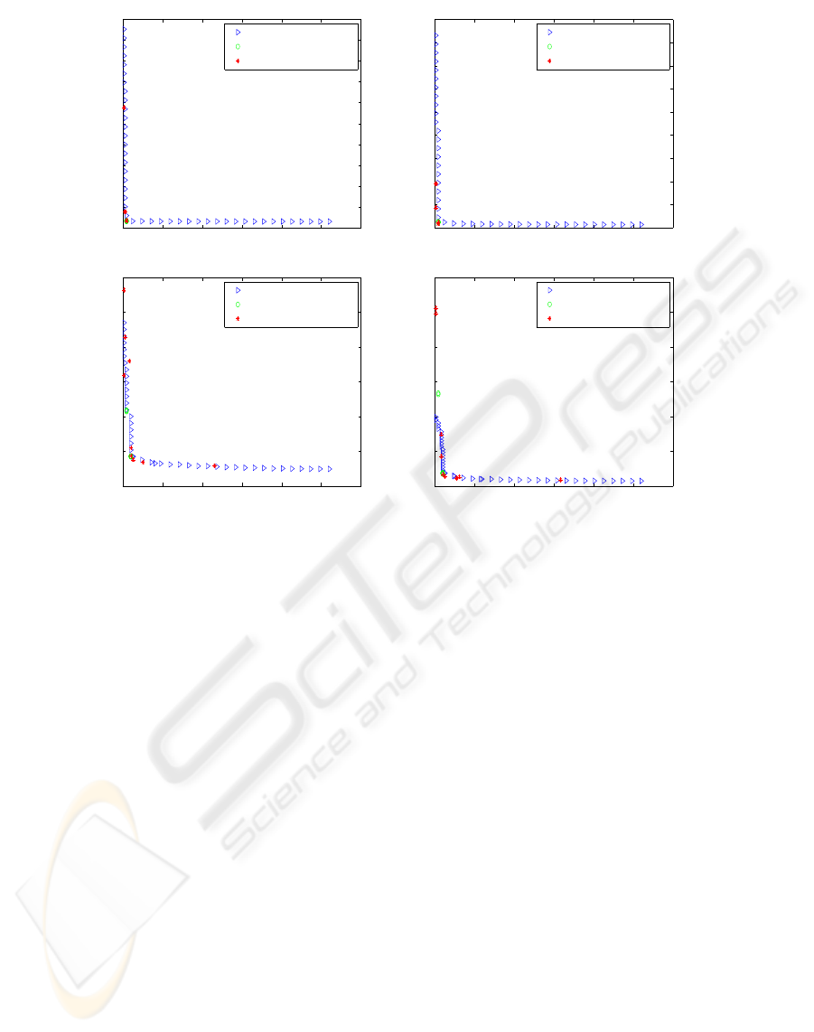
mance. In figure 1 median non-dominated sets ob-
tained for LS-DNSGA are plotted along with the me-
dian performances for different weights considered
for the weighted sum approaches. We separately com-
pared (a) LS-DNSGA and the exhaustive approach
both with the restriction of 2 sensors, and (b) LS-
DNSGA with single objective GA with the number
of sensors allowed to vary.
The non-dominated sets shown in Figure 1 (space
limitations restrict us to only a few time steps) result
in the following observations:
• The weighted sum approach using exhaustive
search finds solutions that only cover a very small
region as compared to LS-DNSGA.
• The weighted sum GA approach is also unable to
cover the entire non-dominated set satisfactorily.
• For all time steps, the weighted sum approach
solutions are mostly dominated, and never better
than those obtained using LS-DNSGA.
• Better results are obtained if the number of sen-
sors is allowed to vary.
For a 2-objectiveproblem, the hypervolume repre-
sents the sum of the areas enclosed within the hyper-
cubes formed by the points on non-dominated front
and a chosen nadir point. Since the objectives are
to be minimized, larger hypervolumes are desirable,
representing better spread and quality of solutions.
We compare LS-DNSGA(with and without popula-
tion seeding) with NSGA-II (with and without pop-
ulation seeding), measuring the average hypervolume
(Padhye et al., 2009) over 51 runs, using the nadir
point (700, 250), based on maximum cost and max-
imum PCRLB values obtained over all time steps.
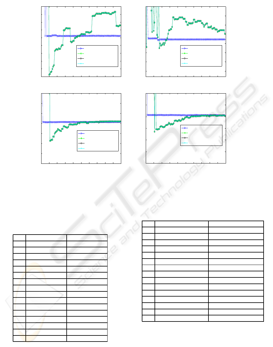
Figure 2 shows that LS-DNSGA is the best per-
former in reaching steady state hypervolume fastest
without showing any oscillations, whereas the other
algorithms convergedmore slowly and sometimes ex-
hibited oscillatory behavior. For all algorithms other
than LS-DNSGA, for time steps 1 and 2, hypervol-
ume starts at a higher value and keeps falling with-
IJCCI 2009 - International Joint Conference on Computational Intelligence
162

0 100 200 300 400 500 600
0
1
2
3
4
5
6
7
8
9
10
Trade−off Solutions at Time Step 1
Cost
PCRLB
LS−DNSGA
Wtd. Approach, 2 sensors
Wtd. GA
0 100 200 300 400 500 600
0
5
10
15
20
25
30
35
40
45
Trade−off Solutions at Time Step 2
Cost
PCRLB
LS−DNSGA
Wtd. Approach, 2 sensors
Wtd. GA
0 100 200 300 400 500 600
0
2
4
6
8
10
12
Trade−off Solutions at Time Step 3
Cost
PCRLB
LS−DNSGA
Wtd. Approach, 2 sensors
Wtd. GA
0 100 200 300 400 500 600
0
5
10
15
20
25
30
Trade−off Solutions at Time Step 4
Cost
PCRLB
LS−DNSGA
Wtd. Approach, 2 sensors
Wtd. GA
Figure 1: Plots for median attainment surface curves for LS-DNSGA along with median performances of weighted summation
approaches for different Ws over first 4 time steps. Plots indicate that LS-DNSGA is able to find a well distributed set of
solutions but the weighted sum approaches can only find few points on the non-dominated set.
out reaching a constant value; this is known to oc-
cur when few, newer and less converged, solutions
replace better but less diverse population members
(Padhye, 2009), (Laumanns et al., 2002).
The improvements in results obtained by LS-
DNSGA are due to the combined effect of local
search and population seeding mechanisms. If the
Pareto front is not changing very rapidly then do-
ing a local search on seeded solutions can lead to
finding of new Pareto front quickly. Although lo-
cal search increases the number of function evalua-
tions in each generation, our simulations showed that
LS-DNSGA was often able to reach steady state re-
quiring fewer function evaluations than other algo-
rithms. Due to space limitations, hypervolume curves
are shown for only a few time steps; the authors can
be contacted for more details.
4.2 Experiment II
Simulations were also carried out to compare the
querying strategies with fixed cost vs. fixed number
of sensors. Three sets of experiments are performed,
with 51 runs for each set. First, the weighted sum ap-
proach was applied and a single objective function F,
was minimized for 11 different values w ∈ { 0.0, 0.1,
0.2, 0.3, 0.4, 0.5, 0.6, 0.7, 0.8, 0.9, 1.0}. Exhaustive
search was conducted with exactly two sensors to be
chosen for querying in each time step. Median Cost
and PCRLB for w = 0.0, 1.0, based on 51 runs, are
listed in Table 2. We then applied LS-DNSGA with
exactly 2 sensors and having minimum PCRLB is se-
lected for querying - this is the ’two sensor strategy’.
Separately, LS-DNSGA was applied, selecting the
solution which has minimum PCRLB and querying
Cost less than 300 units is chosen- this is the ’fixed
cost strategy’. 51 runs of were executed with popu-
lation size 50, maximum generations 100, and muta-
tion probability 0.07, and the 26
th
attainment surfaces
were computed.
For the two-sensor strategy, solutions (with two
sensors) were located on the median non-dominated
front, and the two solutions corresponding to min-
imum Cost and minimum PCRLB are referred to
as ’left’ and ’right’ respectively, and listed in Ta-
ble 3. By comparing these extreme solutions (’left’
and ’right’) with the weighted sum approach solutions
(corresponding to w=0.0 and w=1.0), we can evaluate
whether LS-DNSGA succeeds in find the extrema. In
Table 4 we list the extreme solutions on the entire me-
DYNAMIC AND EVOLUTIONARY MULTI-OBJECTIVE OPTIMIZATION FOR SENSOR SELECTION IN SENSOR
NETWORKS FOR TARGET TRACKING
163

0 10 20 30 40 50 60 70 80 90 100
1000
2000
3000
4000
5000
6000
7000
8000
9000
10000
Hypervolume Curves at Time Step 1
Generations
Hypervolume
LS−DNSGA
No Seeding−LS−DNSGA
NSGA−II
Seeding−NSGA−II
0 10 20 30 40 50 60 70 80 90 100
0.5
1
1.5
2
2.5
3
3.5
4
x 10
4
Hypervolume Curves at Time Step 2
Generations
Hypervolume
LS−DNSGA
No Seeding−LS−DNSGA
NSGA−II
Seeding−NSGA−II
0 10 20 30 40 50 60 70 80 90 100
2000
3000
4000
5000
6000
7000
8000
9000
Hypervolume Curves at Time Step 3
Generations
Hypervolume
LS−DNSGA
No Seeding−LS−DNSGA
NSGA−II
Seeding−NSGA−II
0 10 20 30 40 50 60 70 80 90 100
0
2000
4000
6000
8000
10000
12000
Hypervolume Curves at Time Step 4
Generations
Hypervolume
LS−DNSGA
No Seeding−LS−DNSGA
NSGA−II
Seeding−NSGA−II
Figure 2: Hypervolume Curves for LS-DNSGA with and without seeding, and NSGA-II with and without Seeding for
time steps 1 - 4, under Experiment I, indicating fast and accurate convergence of LS-DNSGA, whereas others are slow in
convergence and their performance levels do not match LS-DNSGA.
Table 2: Optimal Solutions (rounded-off to two decimal
places) obtained by the weighted sum approach using ex-
haustive search (only considering 2 sensors) for w values
0.0 and 1.0
w=0.0 w=1.0
T [Cost, PCRLB] [Cost, PCRLB]
1 9.41, 0.32 9.41, 0.33
2 9.41, 1.21 9.41, 1.23
3 20.36, 1.71 9.41, 4.33
4 20.36, 1.89 9.41, 13.39
5 45.89, 1.59 9.41, 32.22
6 77.85, 2.75 9.41, 61.13
7 70.71, 2.41 9.41, 104.24
8 100.25, 2.20 9.41, 160.77
9 102.61, 2.58 9.41, 240.91
10 100.25, 0.51 9.41, 346.99
11 98.51, 6.16 9.41, 485.67
12 84.21, 23.08 9.41, 662.66
13 84.21, 47.34 9.41, 869.66
14 82.05, 75.76 9.41, 1110.85
15 82.05, 111.06 9.41, 1401.24
dian non-dominated front found by LS-DNSGA us-
ing fixed cost strategy.
From Tables 2 and 3 we observe that values under
left
∗
column are comparable with those under w=1.0.
Similarly, right
∗
column is comparable with w=0.0.
Table 3: Left and Right extreme LS-DNSGA for
twosensorquery
∗
. Rounded-off to two decimal places.
T Left
∗
[Cost, PCRLB] Right
∗
[Cost, PCRLB]
1 9.41, 0.38 9.41, 0.24
2 9.41, 1.75 9.41, 0.96
3 9.41, 3.83 20.41, 1.67
4 9.41, 7.94 20.41, 1.78
5 9.41, 7.37 46.04, 1.44
6 9.41, 10.16 70.97, 2.91
7 9.41, 11.03 80.50, 2.01
8 9.41, 11.03 78.14, 2.57
9 9.41, 12.87 103.00, 2.33
10 9.41, 16.41 103.00, 0.06
11 9.41, 11.03 98.88, 5.08
12 9.41, 41.73 84.52, 20.77
13 9.41, 62.20 84.52, 44.58
14 9.41, 102.56 82.34, 73.23
15 9.41, 143.86 82.34, 107.11
In other words, solutions obtained by LS-DNSGA are
non-dominated (or non-inferior) when compared to
those obtained by the weighted summation approach.
Moreover, for the first few time steps, the sensor pair
that minimizes Cost also minimizes PCRLB, perhaps
due to the positioning of sensors in the field and initial
position of particle. The extreme solutions for cost
constrained LS-DNSGA (with multiple sensor selec-
IJCCI 2009 - International Joint Conference on Computational Intelligence
164

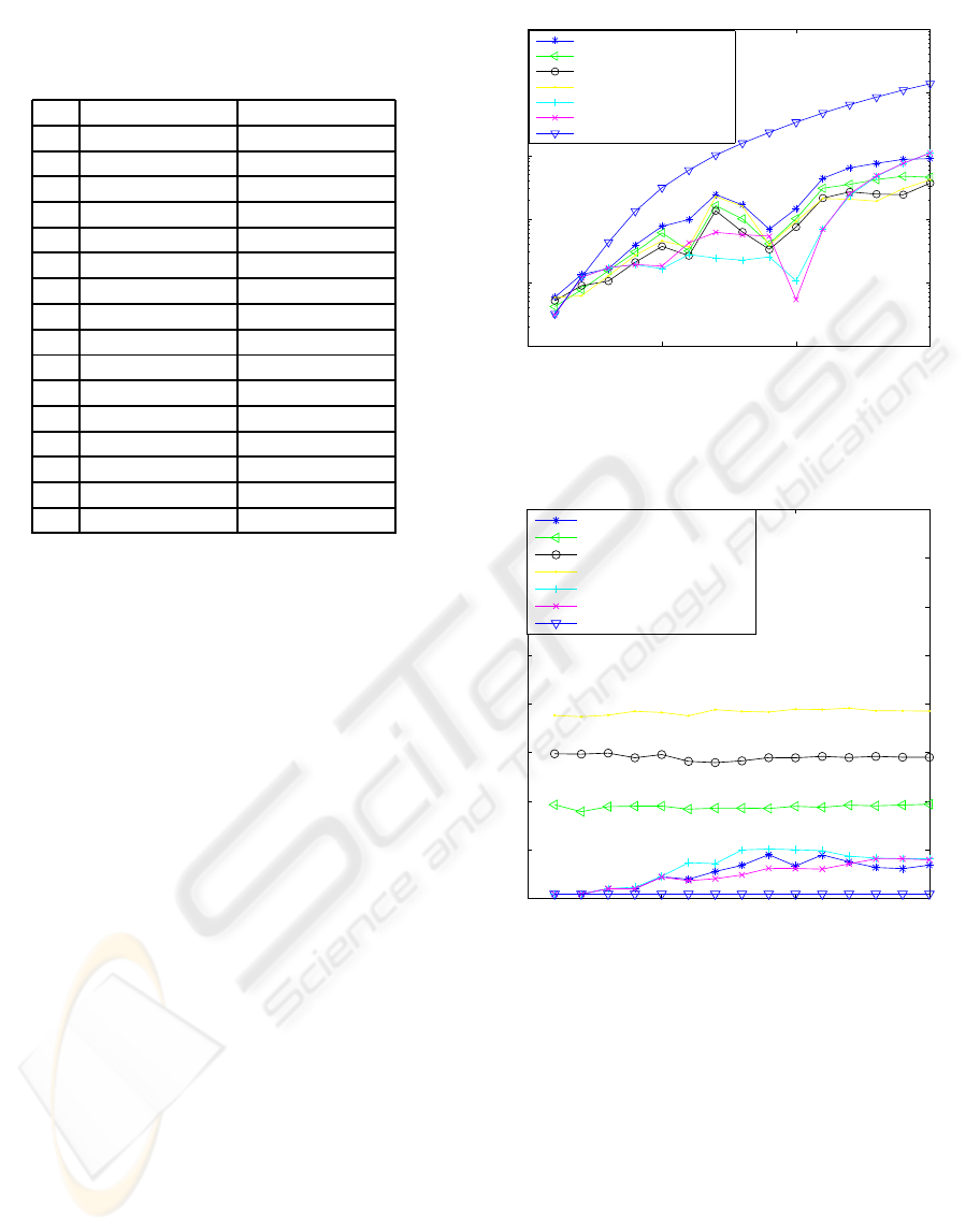
Table 4: Left and Right extreme optimal points obtained by
LS-DNSGA for fixedcoststrategy
∗∗
. Rounded-off to two
decimal places.
T Left
∗∗
Right
∗∗
[Cost, PCRLB] [Cost, PCRLB]
1 3.39, 5.86 520.56, 0.25
2 3.39, 17.01 520.56, 0.63
3 3.39, 5.74 520.56, 0.97
4 3.39, 7.68 520.56, 0.70
5 3.39, 7.47 520.56, 0.70
6 3.39, 8.39 520.56, 0.87
7 3.39, 10.04 520.56, 0.78
8 3.39, 9.77 520.56, 0.73
9 3.39, 10.32 520.56, 1.07
10 3.39, 12.76 520.56, 0.12
11 3.39, 10.48 520.56, 3.40
12 3.39, 25.19 520.56, 10.20
13 3.39, 42.96 520.56, 19.32
14 3.39, 63.93 520.56, 30.51
15 3.39, 103.12 520.56, 45.44
tion), are 1 sensor (min. cost 3.3888 units) and 16
sensors (max. Cost 520.562), computed separately,
which correspond to points on the true Pareto optimal
front.
The M.S.E. in position is plotted against time in
Figure 3 for various strategies. The corresponding av-
erage costs over the time steps are shown in Figure 4,
demonstrating that LS-DNSGA fixed cost (or mul-
tiple sensor) strategies show better performance over
other strategies for most of the time steps (some vari-
ations in performance can be attributed to noise). The
single objective approach with w=1.0, implying min-
imization of cost only, shows the worst performance.
Comparing figures 3 and 4 it can be seen that in-
creased average cost corresponds to a lower MSE.
Further, increasing cost from 300 to 400 units does
not yield a distinguishable improvement in MSE as
compared to change from 200 to 300 units.
The non-dominated solutions obtained for one
simulation and time step 6 are shown in Figure 5. The
optimal point by single objective approach (78.9, 2.7)
with variable number of sensors has lower PCRLB
than the extreme right solution on the non-dominated
solution with fixed number (2) of sensors (32.3, 5.0).
Also, a point on the Pareto front with 3 sensors (72.3,
2.7) dominates the single objective optimal point,
eliminating the latter from the Pareto front, which
leads to the selection of point (32.3, 5.0) as the one
with two sensors and minimum PCRLB value for
querying with multi-objective approach. This shows
why choosing a solution with fixed number of sen-
sors from the entire non-dominated front may lead to
0 5 10 15
10
−1
10
0
10
1
10
2
10
3
10
4
Time Steps
MSE in Position
LS−DNGSA 2 sensors
LS−DNSGA Max. Cost 200 units
LS−DNSGA Max. Cost 300 units
LS−DNSGA Max. Cost 400 units
Single Objective, W = 0.0
Single Objective, W = 0.5
Single Objective, W = 1.0
Figure 3: Comparison of MSE for LS-DNSGA with fixed
number (2) of sensors, LS-DNSGA with Cost Constrained,
and Single Objective Approaches with different weights.
0 5 10 15
0
100
200
300
400
500
600
700
800
Time Steps
Cost
LS−DNSGA 2 sensors
LS−DNSGA Max. Cost 200 units
LS−DNSGA Max. Cost 300 units
LS−DNSGA Max. Cost 400 units
Single Objective, W = 0.0
Single Objective, W = 0.5
Single Objective, W = 1.0
Figure 4: Illustrating the Performance in terms of Average
Cost of LS-DNSGA with fixed number (2) of sensors, LS-
DNSGA with Cost Constrained, and Single Objective Ap-
proaches with different weights.
poor performance, and why the two-sensor strategy
performs worse than the weighted sum approach with
w=0.0 (or 0.5).
4.3 Experiment III
Further experiments were conducted to compare LS-
DNSGA and NSGA-II with varying numbers (30,
40 and 50) of sensors. Hypervolume results are pre-
sented, averaged over 51 runs, for 15 time steps in
Table 5, summarized using ”+”, ”-” and ”o” respec-
DYNAMIC AND EVOLUTIONARY MULTI-OBJECTIVE OPTIMIZATION FOR SENSOR SELECTION IN SENSOR
NETWORKS FOR TARGET TRACKING
165

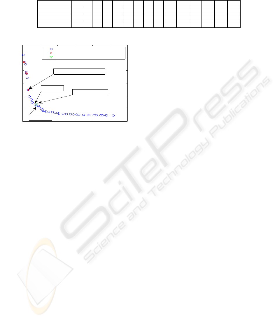
Table 5: LS-DNSGA performance for different sensors over 15 time steps, cost based.
Time Step: 1 2 3 4 5 6 7 8 9 10 11 12 13 14 15
30 Sn. - o + o o o o o o o o o o o o
40 Sn. + - o + o o o o o o + o o o o
50 Sn. - + + + + + + + o o o + + + +
0 100 200 300 400 500 600
0
2
4
6
8
10
12
Cost
PCRLB
Comparison for 16 Sensors, 6th time step
Multi−objective, entire front
Multi−objective, 2 sensor solutions
Single objective, 2 sensor, w=.5
( 32.304699, 4.986475 )
( 77.8524, 2.70 )
3 sensors
4 sensors
Figure 5: Illustration why 2 sensor strategy in multi-
objective can perform poorly.
tively to indicate that LS-DNSGA performance was
better, worse, and almost similar compared to NSGA-
II. Thus, + under time step 2 in third row in table 5 in-
dicates that LS-DNSGA performed significantly bet-
ter in terms of hypervolume over NSGA-II for time
step 2. Similarly o in first row under time step 2 indi-
cates both algorithms performed similarly.
These results show that as the number of sensors
increases, the relative advantage of LS-DNSGA over
NSGA-II increases. Even when the hypervolumesob-
tained were similar, we observed that LS-DNSGA in-
variably reached the steady state hypervolume requir-
ing significantly fewer generations. Seeding and local
search appear to be most helpful in later time steps,
and when the number of sensors is large. Addition-
ally, a single objective approach was also applied to
minimize Cost and PCRLB, separately, and these so-
lutions were found to be often dominated by extreme
solutions obtained by the multi-objective approach.
5 CONCLUSIONS
We have addressed the task of selecting subsets of
sensors (for target tracking) as a multi-objective op-
timization problem, simultaneously minimizing com-
munication cost and PCRLB (providing a bound
on the estimated MSE). A well-known evolutionary
multi-objective algorithm, NSGA-II, was applied to
this problem, along with a new variant, LS-DNSGA,
proposed in this paper. LS-DNSGA was com-
pared against the weighted summation approach and
showed superior performance (faster and accurate
convergence) over NSGA-II, based on median attain-
ment surfaces and average hypervolume. The evo-
lutionary approach was successful in finding a well-
distributed set of tradeoff solutions providing better
decision making as compared to the weighted sum ap-
proach. Two strategies, fixed cost and fixed number
of sensors, were tested and former was found to be
more useful. The proposed algorithm, LS-DNSGA,
was found to perform well on large sensor networks
as compared to NSGA-II, and single objective ap-
proach, highlighting the usefulness of local search
mechanism. Howevwer, local search becomes com-
putationally more expensive when population size in-
creases; future work will explore a probabilistic local
search mechanism.
ACKNOWLEDGEMENTS
This work was supported by the U.S. Air Force Office
of Scientific Research (AFOSR) under grant FA9550-
06-1-0277 during the period May - July, 2009.
REFERENCES
Bar-Shalom, Y., Li, X. R., and Kirubarajan, T. (2001). Esti-
mation with Applications to Tracking and Navigation.
John Wiley and Sons.
Deb, K. (2001). Multi-objective Optimization Using Evolu-
tionary Algorithms. John Wiley and Sons, Dordrecht.
Laumanns, M., Thiele, L., Deb, K., and Zitzler, E. (2002).
Combining convergence and diverisity in evolutionary
multi-objective. Evolutionary Computation, 10:263–
282.
Padhye, N. (2009). Comparison of archiving methods in
multi-objective particle swarm optimization (mopso):
Empirical study. In To appear in Proceedings of the
GECCO conference companion on Genetic and evo-
lutionary computation.
Padhye, N., Juergen, J., and Mostaghim, S. (2009). Empir-
ical comparison of mopso methods - guide selection
and diversity preservation -. In Proceedings of CEC.
IJCCI 2009 - International Joint Conference on Computational Intelligence
166

Rajagopalan, R., Mohan, C.K., Mehrotra, K. G., and Varsh-
ney, P. K. (2005). Proc. 2nd indian int. conf. artifi-
cial intelligence. In An evolutionary multi-objective
crowding algorithm (EMOCA): Benchmark test func-
tion results.
Tichavsky, P., Mauravchik, C. H., and Nehoria, A. (May,
1998). Posterior cram´er-rao bounds for discrete-time
nonlinear filtering. IEEE Transactions on Signal Pro-
cessing, 46(5):1386–1396.
Zuo, L., Niu, R., and Varshney, P. (2006). Posterior crlb
based sensor selection for target tracking in sensor
networks. In Acoustics, Speech and Signal Process-
ing, 2007. ICASSP 2007, pages 1041–1044.
DYNAMIC AND EVOLUTIONARY MULTI-OBJECTIVE OPTIMIZATION FOR SENSOR SELECTION IN SENSOR
NETWORKS FOR TARGET TRACKING
167