SOLVING THE T-JOINT PROBLEM IN RECONSTRUCTING 2-D

OBJECTS

C. Stringfellow, R. Simpson, K. Enloe, R. Krasniqi, T. Ngo, R. Keown

Department of Computer Science, Midwestern State University, Wichita Falls, TX 76308, U.S.A.

J. Hood

Department of Mathematics, Midwestern State University, Wichita Falls, TX 76308, U.S.A.

Keywords: Curve matching, T-joints, Image processing jigsaw puzzles, 2D closed curves and automated reconstruction.

Abstract: This paper describes a solution to the T-joint problem in matching 2D fragments of an object. Matching

fragments of an object is useful for solving puzzles or reassembling archaeological fragments. Many factors,

such as the number of pieces and the complex shapes of pieces make this a difficult problem. Various

approaches to this problem exist. This paper presents an approach to solving the T-joint problem, which

comes up in assembling fragments. The work described in this paper starts with a 2D object that should be

easy to extend to 3D problems.

1 INTRODUCTION

The assembly of fragments of an object using

computer software has significant usages in the real

world. Applications include reconstructing torn

documents or fragmented pottery and artefacts while

excavating ruins of ancient civilizations. It can be a

challenging and formidable task reconstructing an

entire object. A manual approach is time consuming,

especially for a large number of fragments and

requires direct contact with objects, which increases

the chance to damage those artefacts. In contrast, an

automated approach could efficiently reconstruct a

large number of pieces. In addition, the trace of the

reassembly can be kept in an electronic medium for

study.

An additional problem is that in naturally

occurring fragmentation of objects, fragments do not

commonly match at pairs of corners. Most objects

fragment in a way that forms triple junctions, such

as T-joints. McBride and Kimia (2003) reported that

in samples of broken ceramic tiles, T-joints ranged

from 70-89% of the junctions, while other triple

junctions ranged from 6-9%, and non-triple

junctions ranged from 5-20%. Figure 1 shows a T-

joint.

Figure 1: Two puzzle pieces showing T-joint match.

The assembly of the fragments of 3D objects is

complicated. This work focuses on 2D objects,

rather than 3D. In this way, all the drawbacks in 2D

approaches are resolved before leaping to the 3D

world to simplify the computational complexity. In

section 2, previous work on matching objects is

discussed. Section 3 introduces a method to perform

2D curve matching for pieces with T-joints. Section

4 describes the results of processing puzzle pieces

with the method introduced in section 3. Section 5

presents conclusions and future issues to explore.

2 HISTORY REVIEW

Numerous previous works attack matching issues in

reconstructing fragmented objects. Most of them

compare the boundaries of the objects, represented

Stringfellow C., Simpson R., Enloe K., Krasniqi R., Ngo T., Keown R. and Hood J. (2010).

SOLVING THE T-JOINT PROBLEM IN RECONSTRUCTING 2-D OBJECTS.

In Proceedings of the International Conference on Imaging Theory and Applications and International Conference on Information Visualization Theory

and Applications, pages 23-28

DOI: 10.5220/0002824700230028

 SciTePress

by some sort of spline curve (Lee, Clark, & Araman,

2003; Krebs, Korn & Wahl, 1997) or polygonal

approximation. The algorithms split curves at

boundary points and then match sub curves

(Freeman & Garder, 1964; Kong & Kimia, 2001;

McBride & Kimia, 2003; Radack & Badler, 1982;

Stringfellow, Simpson, Bui, Peng, & Hood, 2008;

Weiss-Cohen, Halevi, 2005). Many approaches

perform local shape analysis first, which results in

ambiguous matches and require backtracking to

resolve the mismatches (Freeman & Garder, 1964;

Kong & Kimia, 2001; Radack & Badler, 1982;

Stringfellow, Simpson, Bui, Peng, & Hood, 2008).

Finding accurate matches is more often than not

very time consuming. Curve fitting methods often

require a least squares fit or similar process to

determine the associated error of each fitted curve.

As the number of curves that require processing

increases, the complexity of each fit becomes more

of an issue. This is the situation that is encountered

in the reconstruction of 2D fragmented objects.

Each collection of N fragments, where each

fragment has on the average M distinct edges,

requires O((MN)

) curve fits. Of course, problem

specific information can be used to reduce this

number.

The approaches used by researchers vary based

on the characteristics of the fragmented objects.

These characteristics concern orientation of pieces,

whether there are missing pieces, whether the

exterior boundary is known beforehand (such as a

rectangular grid), whether there is a unique solution,

and what types of junctions between pieces are

allowed (Kleber, 2009). Some approaches consider

image features of the pieces, such as color and

texture (Nielsen, Drewsen, & Hansen, 2008) and

others consider shape of pieces (Da Gama Leitao &

Stolfi, 2002; Freeman & Garder, 1964; Goldberg,

Malon, & Bern, 2002; Horst & Beichl, 1996; Krebs

et al., 1997; Kong & Kimia, 2001; Lee et al., 2003;

McBride & Kimia, 2003; Radack & Badler, 1982;

Stringfellow et al., 2008; Zhu, Zhou & Hu, 2008),

while (Weiss-Cohen & Halevi, 2005; Yao & Shao,

2003) consider both.

Many of the approaches have problems. Freeman

and Garder (1964) repeatedly search all pieces and

the best matches are merged to form new pieces

until only one piece is left. Insufficient constraints

result in mismatches and require backtracking. The

algorithm by Goldberg et al. (2002) is efficient, but

not fully automated and only works on pieces with

four corners. Yao and Shao (2003) present no

method to solve for triple junctions.

Kong and Kimia (2001) McBride and Kimia

(2003) and Zhu et al. (2008) present two-step

approaches to solving reconstruction of fragmented

objects. In both, the first step finds likely candidate

pairs of pieces by computing affinity measures using

polygonal approximation of pieces. In Kong and

Kimia (2001) McBride and Kimia (2003) triples that

arise from generic junctions (Y- and T-joints) are

formed from this rank-ordered list of the top-ten

pairings. Their second step compares these

candidate pieces at a finer level. If a match, the

pieces are merged and removed from the piece list

and the merged piece is inserted. The results show

some mismatches, probably due to issues in the

second matching step. In Zhu et al. (2008) the

second step uses a confidence number assigned to

each pair and then maximizes the consistency until

the confidence reaches one. This creates the

advantage of overall checking of joins to decide on

matches or false positives. However, it only results

20-30 percent matches.

Stringfellow et al. (2008) present a method that

works on pieces with discrete closed boundaries,

represented by points (not curves or polygonal

approximations). It does not require pieces to fit a

grid. It does not match pieces with T-joints, but

pieces may “join” a puzzle, if an adjacent edge

without a T-joint is matched to another different

piece. It does require a very small amount of user

interactions to verify automated results.

3 METHOD

This paper builds on the work of Stringfellow et al.

(2008) to solve the T-joint problem. The approach,

which is now a 2-step matching process is briefly

described.

First, boundary points representing outlines are

extracted from scanned images of puzzle pieces.

Then the convex corner points are detected using a

non-parameterized algorithm (Staples & Hood,

2008). In order to match curve segments of pieces, a

fitness function is introduced to determine whether

two curve segments are candidates for matching.

Figure 2 shows the curve segment is divided into

four small segments. It also shows the start points

and end points for the four sub-segments. The

middle point of a segment is chosen to divide the

segment into sub-segments. The distance lengths of

the sub-segments are denoted d

- d

, respectively.

The four sub-segments form three angles Ө

, - Ө

The distance of a segment is computed in two ways:

the number of pixels between start and end points

IMAGAPP 2010 - International Conference on Imaging Theory and Applications

denoted as PD and the straight line distance between

start and end points and is denoted as D. The fitness

value, F(S

), is calculated using absolute or

relative differences between the nine criteria. The

smaller the fitness value, the better chance the two

segments are actually a match. If the fitness is too

large, then the pair is rejected as a candidate pair.

Figure 2: Break down of a curve segment in order to

calculate its fitness value.

Other tests are applied to determine if the mid-

points and quarter points of segment S

and segment

are close to each other after a rotation and a

translation are performed. If they are too far away

from each other, then the fitness F(S

) is set to a

large value (not a candidate for matching pair.)

Figure 2 shows two original segments and the

segments after a rotation and a translation.

Figure 3: S

and S

and their sub-segments before and after

a rotation and translation.

Next, the algorithm (shown in Figure 4) uses a

local approach to match curves. The algorithm

selects a puzzle piece with four or more corners. If

there is no piece with four or more corners, the

algorithm selects just any piece. However, the more

corners a piece has, the better the matching pool

generated. Next, pieces with the matches for the

piece’s curve segments are found and the adjacent

pieces are pushed onto a stack. The next piece out of

the stack is popped and the best match for its curve

segments is found. The process is repeated until the

stack is empty.

Figure 4: Regular curve matching algorithm (Stringfellow

et al., 2008).

After regular curve matching, T-joint matching

is performed. The unmatched segments are sorted

(by length) into a list. The T-joint algorithm (shown

in Figure 5) starts with a unmatched pair of

segments selected from the sorted segment list. It

calculates a sub-segment in the longer segment equal

in length to the shorter segment starting at the start

point of the longer segment and applies the matching

criteria to see if they are a match. If not, it

calculates a sub-segment in the long segment

starting at the finish point and determines if they are

a match. If a match is found (from either end point),

it subdivides the long segment into a matched (sub)

segment and a leftover (sub) segment. The leftover

segment is inserted into the sorted segment list for

future consideration.

Figure 5: T-joint matching algorithm.

push piece [i] in the stack

while the stack is not empty

pop (current_piece )

for every segment of current_piece

find the best fit segment

if there is a match and the adjacent piece

with the best fit is not in the stack already

move adjacent piece to new position

ush the adjacent piece onto the stac

1: Get distance of short segment.

2: Find sub-segment in long segment that is equal

length to short segment starting at the start

point of long segment.

3: The new sub-segment is separated into 4 (equal)

segments: calculate the midpoint and quarter

points and other matching criteria.

4: Compare the sub-segment to the short segment to

see if they match using the criteria.

5: If they match by a certain fitness value, then

compute the left over part of the long segment.

6: If segments do not match, create a sub-segment

from the long segment with same distance as

short segment starting at finish point of long

segment.

7: Perform Steps 3-5 for this sub-segment.

8: If either of the sub-segments of the long segment

match the short segment, compute the left over

segment of the long segment.

9. The matched sub-segment is removed from the

segment list and the leftover segment is inserted

in th

e sorted segment list

SOLVING THE T-JOINT PROBLEM IN RECONSTRUCTING 2-D OBJECTS

The criteria for determining if segments are

matches in regular matching and T-joint matching

are essentially the same, except segment length

criteria is disregarded in the overall fitness value for

T-joint matching (since the segments compared are

made to be the same length). The tolerance values

for the criteria can be made different for T-joint

matching, but with these puzzles they were left the

same. Only the overall fitness value was decreased

in the T-joint matching (to compensate for the

segment length criteria).

Overall, regular and T-joint matching is O(S

where S is the number of segments in all the pieces.

Some efficiency is gained in regular matching, by

only comparing segments to segments of other

pieces, as long as those segments are within its

neighbourhood in the sorted list. (A neighbourhood

is size 10.) In addition, if the differences between

two segments in one of the nine criteria are too

large, then no other comparison calculations are

performed. When a pair of segments is matched, a

piece gets attached to the puzzle, and that piece

becomes the current piece for further matching. If a

piece has none of its segments match, the algorithm

goes back to a previous piece and checks its

remaining unmatched segments. It is possible to

join an N-piece puzzle with O(N) segment matches.

The worst case scenario is that no pieces match, and

O(S

) segments are compared. After regular

matching is performed, the unmatched segments are

stored in a sorted unmatched segment list – this

takes O(S). The T-joint algorithm, worst case,

would need to compare every unmatched segment to

every other unmatched segment twice – taking

O(S

), but if regular matching found most of the

matches, there would be fewer unmatched segments

in the sorted list to compare.

4 RESULTS

The application was developed using C# within the

Microsoft Visual Studio.Net 2005 platform. Puzzle

pieces were scanned in using a HP ScanJet 5200C

scanner, several pieces at a time. RGB format is

transformed to greyscale and then the images are

converted to a binary format, so all pixels are either

black or white. Boundaries are extracted and corner

points are detected, then regular matching is

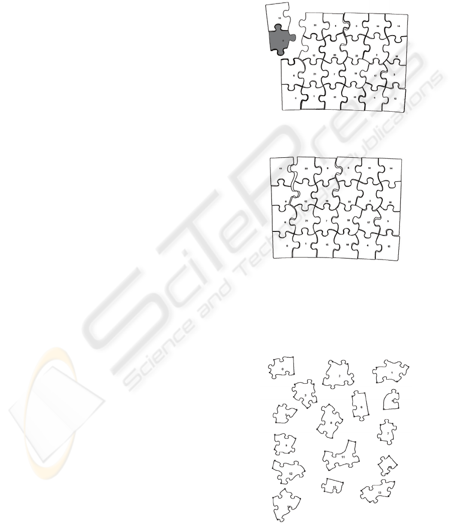
performed. Figure 6 shows a puzzle put together

after regular matching is performed. The two pieces

not joined only have segments with T-joints. There

are a few pieces joined in the puzzle that have

segments with T-joints, but they are matched to

other pieces using segments without T-joints.

Figure 7 shows the results after the T-joint

matching is performed. The bottom segment of the

shaded piece is matched to the joined puzzle. (There

is a bit of round-off error in the translation and

rotation of pieces.)

Figure 6: Puzzle after regular matching performed

(Stringfellow et al., 2008).

Figure 7: Final result after T-joint matching.

Figures 8 – 10 show a puzzle with many T-joints.

As can be seen in Figure 11, only 2 pairs of pieces

are matched using regular matching. After the T-

joint matching algorithm is applied, every piece is

joined to the puzzle.

Figure 8: Puzzle 2 with many T-joints.

IMAGAPP 2010 - International Conference on Imaging Theory and Applications

Figure 9: Puzzle 2 after regular matching.

Figure 10: Puzzle 2 after T-joint matching performed.

Figures 11 and 12 show a puzzle that has pieces

with smoother, longer curves and many T-joints.

All pieces are matched by the T-joint matching

algorithm. Note that this puzzle has joints where

two pieces match, but do not have either a start or

end point in common (designated as a Type 3

junction in [8]).

Figure 11: Puzzle 3 after regular matching is performed.

Figure 12: Puzzle 3 after T-joint matching performed.

Figures 7, 10 and 12 show that the algorithm in

Figure 5 is successful in putting the remaining

puzzle pieces with T-joints together. This algorithm

also solves the problem of type 3 junctions. These

joints get resolved when the piece’s segment is

divided into a matched part (to another piece) and a

leftover part that is then inserted into the segment

list to be matched with a future piece. The type 3

joints reduce to T-joints. In this way, the semi-

circular piece in puzzle 3 is matched to three pieces.

The threshold values for some of the fitness

criteria for a match were made stricter (that is, the

difference between two segments’ criteria had to be

smaller to be considered a match. In puzzles 1 and

2, the criteria had to be relaxed in order to get them

completed. There is a trade-off between using

stricter criteria and the number of correct matches.

When the criteria was made more strict, fewer

matches were made (although not much fewer), but

it did not give fewer false matches, except in puzzle

2. In puzzle 3, a large number of the false T-joint

matches were due to the semi-circular piece, which

tended to match a lot of other arcs in other pieces’

segments.

False T-joint matches are more likely than false

regular matches, due to the fact that two criteria are

eliminated. (The T-joint matching algorithm makes

pixel segment length and actual segment lengths the

same.) Making the remaining criteria tighter, may

result in fewer false T-joint matches, but it may also

reduce true T-joint matches.

5 CONCLUSIONS AND FUTURE

WORK

This paper proposes a method and its

implementation for semi-automatic reconstruction of

2D jigsaw puzzles that have pieces with T-joints.

SOLVING THE T-JOINT PROBLEM IN RECONSTRUCTING 2-D OBJECTS

Applied to a 24 piece puzzle, the implemented

application is able to put all 24 pieces together.

Puzzles 2 and 3 are also entirely put together.

Efficiency in this approach is achieved in several

ways. First only pairs of segments nearby in the

sorted list of segments are compared during regular

matching, and only if they meet the other distance

and angle criteria do they undergo more

calculations. T-joint matching is only performed on

unmatched segments after all regular matching is

done. Type 3 junctions reduce to T-joints after

matched segments are subdivided into matched and

leftover segments.

The suggested approach is considered a

successful and reliable one. This approach

reconstructed all the pieces of a given set of objects.

Restricting the fitness criteria may reduce the

number of matches and increase the number of false

matches, but it still results in successful matching.

Future work needs to be done to base the fitness

criteria on properties of the fragments, such as their

size.

Future research will also consider matching

combined pieces. By applying this approach, there

exists a potential to resolve any few remaining

unmatched pieces. Applying this approach to the

reconstruction of ancient artefacts would result in

considerably less pieces having to be touched over

and over again.

Finally, for the jump to 3D, the work will likely

follow a similar technique to Krebs et al. (1997)

using 2D slices of 3D objects, although rather than

using splines the approach will consider the points in

a cloud to represent the edges or boundaries of the

object.

REFERENCES

Da Gama Leitao, H., Stolfi, J., Sept 2002. A Multiscale

Method for the Reassembly of Two-dimensional

Fragmented Objects. In Trans. On Pattern Analysis

and Machine Intelligence. vol. 24, pp. 1239-1251.

Freeman, H., Garder, L., 1964. Apictorial Jigsaw Puzzles:

The Computer Solution of a Problem in Pattern

Recognition. In IEEE Trans.Elec. Comp., vol 13, pp.

118-127.

Goldberg, D., Malon, C., Bern, M., June 2002. A Global

Approach to Automatic Solution of Jigsaw Puzzles. In

(SoCG’02). Proc. of Symposium on Computational

Geometry, pp. 82-87.

Horst, J.A. and Beichl, I., June 1996. Efficient Piecewise

Linear Approximation of Space Curves Using Chord

and ARC Length. In Proc. of the Society of

Manufacturing Engineers Applied Machine Vision.

Kleber, F., Sablatnig, R., July 2009. A Survey of

Techniques for Document and Archaeology Artefact

Reconstruction. In Int’l Conf. on Document Analysis

and Recognition, pp. 1061-1065.

Kong, W., Kimia, B., Dec. 2001. On Solving 2D and 3D

Puzzles Using Curve Matching. In IEEE Computer

Society Conf. on Computer Vision and Pattern

Recognition, pp.583-590.

Krebs, B., Korn, B., Wahl, F.M., Oct.1997. 3D B-spline

Curve Matching for Model Based Object Recognition,

In Proc. of Int’l Conf. on Image Processing, pp. 716-

719.

Lee, S., Abbott, A.L., Clark, N., Araman, P., Nov. 2003.

Spline Curve Matching with Sparse Knot Sets:

Applications to Deformable Shape Detection and

Recognition. In Proc. of the 29th Annual Conf. of the

IEEE Industrial Electronics Society, pp. 1808-1814.

McBride, J., Kimia, B., June 2003. Archaeological

Fragment Reconstruction Using Curve-Matching. In

(CVPRW’03), Proc. of Conf. on Computer Vision and

Pattern Recognition Workshop, pp. 1-8.

Nielsen, T., Drewsen, P., Hansen, K., Oct. 2008. Solving

Jigsaw Puzzles Using Image Features. In Pattern

Recognition Letters. vol. 29, no. 14, pp. 1924-1933.

Radack, G., Badler, N., Jigsaw Puzzle Matching using a

Boundary-Centered Polar Encoding, CGIP, vol 19,

1982, pp. 1-7.

Staples, J., Hood, J., Nov. 2008. Deparametrization of a

Discrete Convex Corner Detection Algorithm. In

(CAINE’08) Proc. of Computers and Their

Applications in Industry and Engineering, pp. 180-

184.

Stringfellow, C., Simpson, R., Bui, H., Peng, Y., Hood, J.,

Nov. 2008. Matching 2D Fragments of Objects, In

(CAINE’08) Proc. of Int’l Conf. on Computers and

Their Applications in Industry and Engineering, pp.

150-156.

Weiss-Cohen, M., Halevi, Y., Nov. 2005. Knowledge

Retrieval for Automatic Solving of Jigsaw Puzzles. In

Proc. of Int’l Conf. on Computational Intelligence for

Modeling, Control and Automation, and Int’l Conf. on

Intelligent Agents, Web Technologies and Internet

Commerce, pp. 379-383.

Yao, F., Shao, G., Aug. 2003. A Shape and Image

Merging Technique to Solve Jigsaw Puzzles. In

Pattern Recognition Letters. vol. 24, no. 12, pp. 1819-

1835.

Zhu, L., Zhou, Z., Hu, D., Jan. 2008. Globally Consistent

Reconstruction of Ripped-Up Documents. In IEEE

Trans. On Pattern Analysis and Machine Intelligence,

vol. 30, no. 1, pp. 1-13.

IMAGAPP 2010 - International Conference on Imaging Theory and Applications