ON SOME PECULIARITIES OF CLUSTER ANALYSIS
OF PERIODIC SIGNALS
V. Znak
The Institute of Computational Mathematics and Mathematical Geophysics SB RAS, Pr. Lavrentieva 6, Novosibirsk, Russia
Keywords: Cluster analysis, Analysis of periodic signals, Extraction of signals.
Abstract: An important task of geophysical research is in the answer to the question about the quality of signals, i.e.,
estimating the locus of the signal and the degree of their presence in noises. Such indications determine the
degree of trust to consequent estimations (e.g., estimations of wave arrival times). As seismic data are
periodic signals in their nature, conventional means for examining such signals are Fourier and spectral
analyses. However, this method does not allow us to clear up questions about probability of signals presence
and their locus in the recorded data. We consider another approach – the cluster analysis of periodic signals,
propose the formal conditions which must be satisfied by a period of signal existence, and give some results
of analysis of real data recorded in field conditions.
1 INTRODUCTION
The prompting motive of our research is the needs in
noisy geophysical data analysis. The basis of such
data is periodic (harmonic or frequency-modulated)
signals recorded at discrete instants of time.
However, the corresponding signals are widely used,
and an appropriate research can be of interest in
other fields of activity.
In practice, geophysical data are recorded in field
conditions. The point is that in the process of wave
propagation and in recording data one or another
type of errors takes place. Therefore, analysis of
such data demands a special attention. Usually, in
this case researchers attract a harmonic (I. I.
Gurvich, and G. N. Boganic, 1980) or a spectral
analysis (E. A. Davidova, and others, 2002).
However, an appropriate approach cannot decide the
dilemma “time-frequency” (the spectrum
components are listed in a domain, where the time
scale is absent).
Currently, methods of wavelet analysis and
transformation (A. A. Nikitin
, 2006, E. Baziw, 1994)
are of interest to researchers. Here, time localization
of the signal frequency components can be found.
Essentially, such an approach is an analog to
convolution or linear concordant filtration, or, in
other words, it is a development of the window
Fourier analysis.
We will treat periodic signals as time series and
consider another approach, based on the cluster
analysis. To the best of our knowledge, the notion of
a cluster is used by few of authors to analyze
periodic signals (Znak V. I. and Grachev O. V.,
2009).
2 METHODOLOGY OF CLUSTER
ANALYSIS OF PERIODIC
SIGNALS
We can treat the time evolvent of a periodic signal
on a plane as a specific image, and set a problem of
studying some or other its features. However, such
an image becomes considerably complicated in the
presence of noises.
The problem can be simplified if an image of
some integrated estimation of a signal is used as an
object of analysis. Here, we offer to employ an
estimation of a standard deviation (dispersion) on
some running basis. The behaviour of such
estimations as time function σ (t) will reflect the
energy distribution of a signal in the region of their
existence. Then, the evolvent of function σ (t) on a
corresponding 2-D plane can be considered as an
image of a cluster formation. Features of such an
image are of interest for the purposes of analysis of
periodic signals.
226
Znak V. (2010).
ON SOME PECULIARITIES OF CLUSTER ANALYSIS OF PERIODIC SIGNALS.
In Proceedings of the 7th International Conference on Informatics in Control, Automation and Robotics, pages 226-229
DOI: 10.5220/0002911502260229
Copyright
c
 SciTePress

As the above estimation we use
/LLMxLσtσ
Lj
jk
∑
∈
−==
2
))(()()(
(1)
where L is odd, x is signal values, j=(L-1)/2,…, N–
(L–1)/2 (N is a signal length). We will assume σ(t) is
integers.
Let
σ
ˆ be the uppermost dispersion value: 0 ≤ σ
k
≤
σ
ˆ and t
k
is an instant of time. Then, some integer
h (0≤h≤
σ
ˆ ) will be called a "threshold". Thus, we
juxtaposed with our signal estimations a grid h
l
×σ
k
on a 2-D plane, which will be denoted as Q: h=0,…,
σ
ˆ ; k=(L-1)/2,…, N–(L–1)/2). Further, we will
suppose that each point of the grid represents an
event q
k
(h) ∈ Q, where q∈(0,1):
. if ,0
, if,1
)(
lk
lk
k
h
h
hq
<
≥
=
σ
σ
(2)
For any threshold h, the respective subset
Q
r
(h)⊂Q for the adjacent instants will be called a
cluster if for all the events q
k
of Q
r
(h) the
corresponding σ
k
is greater or equal to the h, i.e.:
∀q
∈Q
r
(h): q=1. The cardinal number of such cluster
is
)(,...,1 ,)(
)(
hmrqh
hQq
r
r
==
∑
∈
β
(3)
and locus in time is Δt
r
(h) = t
1(r)
(h) ÷ t
n(r)
(h).
Naturally, both the quantity of such clusters and
the cardinal number of each cluster depend on the
threshold value.
We can speak about two clusters of the two
neighboring thresholds that a cluster Q
s(r)
(h+1) is a
child of Q
r
(h) if they are intersecting in time:
Δt
r
(h)&Δt
s(r)
(h+1) ≠ 0. We will pool such clusters
and call them a cluster family. The cardinal number
of this cluster family is
∑
=
++=
)(
1)(
)(
)1()()(
rn
rs
rsrr
hhhb ββ
(4)
etc. Let
∑
=
=
)(
1
)()(
hm
r
r
hbhB
(5)
be a common cardinal number of cluster families on
the threshold h. Then the relation
)(/)()( h
B
hbh
P
rr
=
(6)
will be called a representative probability of the
family Q
r
(h).
Let us consider a series of functions P
r
(h),
r=1,…, m(h), h=1,…,
σ
ˆ . We expect that the
behavior of such functions reflects the degree of the
presence of a signal in noise. At the same time, they
are tied to subjects, which have their own locus in
time.
The matter of the problem is to investigate the
behaviour of these functions for answering the
questions about the degree of the presence of a
periodic signal in noise, and its locus in noisy data.
3 ON STUDING THE SIGNAL
EXISTENCE
Let us consider some cluster formation σ
k
(L) as an
image ℵ under condition of any running basis L
(Fig. 1).
Figure 1: An example of the mapping of the dispersion
estimations with a running basis.
Now, turn to the question about picking out the
most informative threshold with regard to a
representative probabilities. For answer on the
question, we will study situations beginning from
threshold h=0. However, first of all, we will make
some remarks based on the nature of a signal in
question. We suppose:
1) A process of signal recording in time (t=0)
begins before a signal arrival, i.e., T
0
>0, where T
0
is an instant of a signal arrival time.
2) A signal on the dispersion estimator input is
y=s+
ξ , where s is a source signal, and ξ is an
additive white noise with zero mean Gaussian
distribution. Let t
N
be a signal recording period,
and ΔT a signal existence period. Then, the
following conclusion is a consequence of such
supposition: the probability of localizing the
uppermost dispersion value k(
σ
ˆ ) on ΔT is
proportional to the ratios t
N
/ΔT and to the signal-
to-noise ratio, i.e., P(
σ
ˆ (k)∈ΔT) ∼ t
N
/ΔT & s/ ξ =
f(t
N
/ΔT, s/ ξ ). (a more exact dependence needs a
separate attention).
ON SOME PECULIARITIES OF CLUSTER ANALYSIS OF PERIODIC SIGNALS
227

Now, we will study a cluster families beginning
with threshold h
0
= 0. We can say, that the threshold
h
0
=0 is non-informative for us because we have
t
1
(0)=0 for a single clusters family Q
1
(h
0
)
(obviously, P
1
(h
0
)= 1.0). We can say the same with
regard to the threshold h
1
=1 if the same conditions
t
1
(h
1
)=0 for single Q
1
(h
1
) (P
1
(h
1
)=1) are fulfilled,
and so on.
Let, for the first time in threshold raising, h
l
be
such a threshold, where t
1
(h
l
) > 0 for m(h
l
) ≥ 1. In
this case, we will have the three sets: 1) a set of
instants of time of the beginning of cluster families
t
1(r)
(h
l
), 2) a set of periods of existence of the
appropriate cluster families Δt
(r)
(h
l
), and, 3)
representative probabilities of the appropriate
families P
r
(h
l
) (r=1,…, m(h
l
)).
Here, the following conditions are fulfilled:
i) one (or more) of such instant of time at which the
condition t
1(r)
(h
l
)>0 is fulfilled;
ii) a set of probabilities includes such P
r
(h
l
), that the
condition P
r
(h
l
)=max is fulfilled;
iii) a set of periods of existence of cluster families
includes such Δt
r
(h
l
) that the condition
t(
σ
ˆ )∈Δt
r
(h
l
) is fulfilled (1≤ r ≤m(h
l
)).
We will suppose that a locus of signal existence
is reflected by such a period of existence of the
cluster family Δt
r
(h
l
), which fulfils (obeys) the
following conditions:
(7)
where Δt
r
(h
l
) is t
1(r)
(h
l
) ÷ t
n(r)
(h
l
).
4 AN EXAMPLE OF STUDING A
SIGNAL
The methodology in question was used for analysis
of data recorded in the course of monitoring (in
2007) of the Karabetov mud volcano on Mt. of
Taman Province (data recorded by Z-component of
receivers for profile line T1, results of field
experiments are currently accessible on the web_site
http://opg.sscc.ru). Seismic (or vibro-) records
were recorded from 10 T vibratory source with a
frequency band of 10–64 Hz, and with a sampling
frequency = 0.004 sec. Appropriate data can be
found at http://opg.sscc.ru/db.
The results obtained are given in the Table 1.
The columns of this Table include distances between
a vibratory source and a receiver (S), h
min
÷h
max
=
σ
ˆ ,
periods of existence of the appropriate cluster fami-
lies t
1
÷t
2
, and appropriate estimations of
representative probabilities (P) for running basis
Table 1: Estimations of signal locus in time.
S m. L h
min
÷h
max
t
1
÷t
2
P
2363 25 6÷415 3933÷19988 0.94
75 14÷396 3689÷15669 0.89
125 16÷390 1520÷14247 0.91
2415 25 9÷305 2041÷19502 0.95
75 16÷292 2284÷19672 0.96
125 28÷279 3901÷9316 0.81
2461 25 13÷156 3173÷9917 0.45
75 24÷133 3190÷10305 0.50
125 27÷121 3210÷10471 0.52
2557 25 3÷64 3315÷19988 0.90
75 6÷53 3481÷19963 0.92
125 6÷46 3455÷19938 0.92
2601 25 5÷165 4045÷19988 0.88
75 11÷151 4060÷18122 0.85
125 15÷132 3741÷18114 0.88
2647 25 8÷98 3493÷8855 0.42
75 12÷88 3593÷14414 0.73
125 14÷86 2213÷13365 0.77
2698 25 2÷13 8642÷19988 0.73
75 3÷13 8832÷19963 0,77
125 3÷13 8807÷19938 0.77
2749 25 6÷87 1410÷12065 0.59
75 8÷84 1150÷19963 0.98
125 9÷82 1170÷19938 0.99
2796 25 6÷87 2637÷15919 0.89
75 10÷78 972÷15800 0.98
125 10÷71 360÷16047 0.99
2845 25 15÷111 3508÷10413 0.58
75 21÷105 569÷11594 0.82
125 22÷100 898÷11615 0.83
2894 25 6÷51 3897÷18815 0.89
75 9÷46 3889÷15243 0.88
125 10÷43 3863÷11205 0.59
2999 25 5÷76 9532÷19988 0.51
75 8÷67 9573÷19963 0.5
125 8÷56 1824÷19938 0.96
3046 25 6÷60 5646÷19988 0.80
75 8÷52 2209÷19963 0.97
125 8÷47 2185÷19938 0.97
3095 25 5÷111 3987÷19988 0.93
75 7÷90 3988÷19963 0.95
125 7÷76 3963÷19938 0.95
3141 25 12÷67 3665÷11019 0.65
75 17÷61 3838÷9707 0.71
125 18÷54 4054÷9388 0.74
3198 25 12÷74 4945÷19988 0.81
75 `8÷66 6011÷9346 0.43
125 18÷64 4288÷19938 0.87
),()
ˆ
(
max,)(
,0)(
)(1
lr
lr
lr
htt
hP
ht
Δ∈
=
>
σ
ICINCO 2010 - 7th International Conference on Informatics in Control, Automation and Robotics
228

L∈{25, 75, 125}.
Estimations of signal locus in time for S∼0 m are
given in the Table 2 (all the representative
probabilities are equal to 1).
The processing and analysis data were obtained
by means of interactive computer system of
designing and support of one-dimensional weighed
order statistics filters (
V. I. Znak, 2009).
Table 2: Estimations of signal locus in time for S∼0 m.
L h
min
÷
h
max
t
1
÷t
2
25 6÷415 3870÷18883
75 14÷396 3846÷18908
125 16÷390 3821÷18933
By way of example, an image of investigated
signal (for S=2647 m) and appropriate dispersions is
shown in Fig. 2.
Figure 2: An image of signal and appropriate dispersions
for L=25, L=125 (S=2647 m).
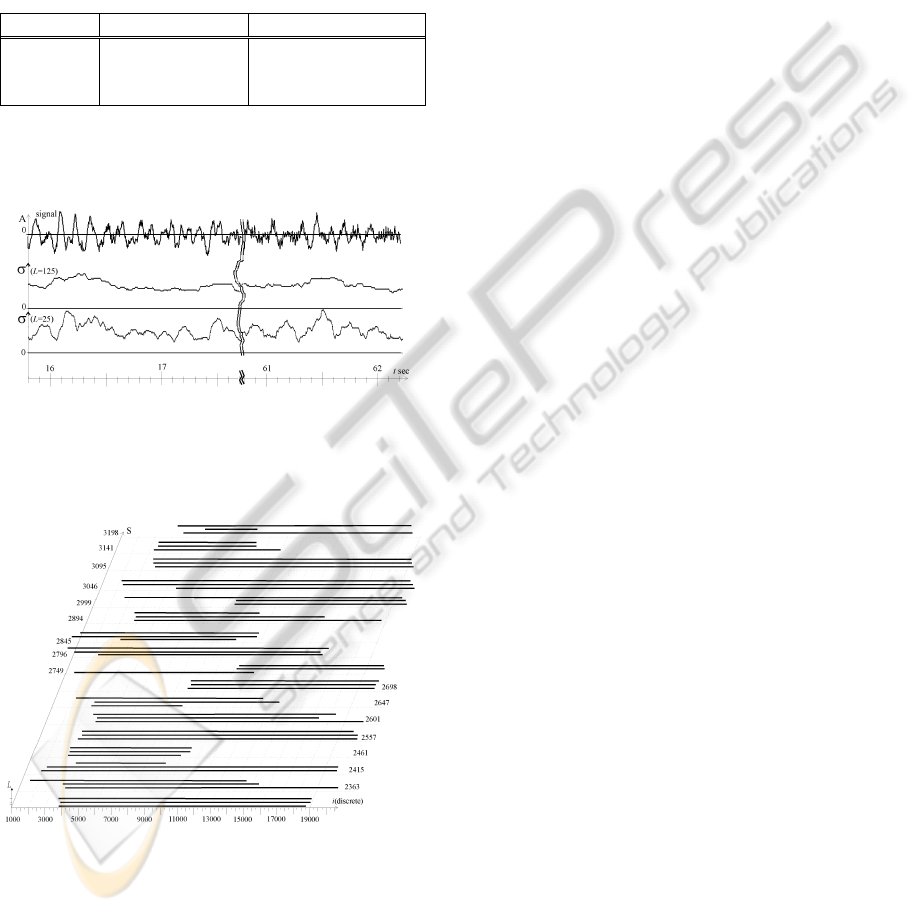
Estimations of the data from the Table 1 are
given in Fig. 3.
Figure 3: Estimations of the time locus of the signal for
running basis L∈{25, 75, 125} and for different distances.
5 CONCLUSIONS
We have considered the approach of cluster analysis
of periodic signals, proposed the formal conditions
which must be satisfied by a period of signal
existence, and given some results of analysis of real
data recorded in field conditions. Analysis of the
results obtained by studying real signals allows us to
say that the approach in question can result in close
estimations of a locus in time of a pure signal, and in
less close estimations of a locus in time of noisy
signals.
Our main objective was restricted by
development of the method of formalized analysis of
periodic signals for estimation of their period of
existence. We have not concerned methods of
improving signals as it is a theme of separate
investigation. We suppose that more exact decisions
can be attained by attracting analysis of the left and
the right uniformity of cluster families (Znak V. I.,
2009) and frequency processing (Znak V. I., 2005).
Cluster families, which reflect a locus of a signal on
its boundaries, must have a higher uniformity than
for others.
The work is supported by the grant 09-07-00100.
REFERENCES
Gurvich I. I., Boganic G. N., 1980. Seismic research.
Moscow, “Nedra” (in Russia).
Davidova E. A., Copilevich E. A., Mushin I. A., 2002.
Spectral-time method for a mapping of types of
geological layers, Reports of RAS, 385(5), pp. 682-
684, (in Russia).
Nikitin A. A., 2006. New tricks of geophysical data
processing and their well-known analogous.
Geophysics, No 4, pp. 11-15 (in Russia).
E. Baziw, 1994. Implementation of the Principle Phase
Decomposition Algorithm,” in Proc. IEEE
Transactions on signal processing. July 2007 45 (6),
1775–1785.
Znak V. I., and Grachev O. V., 2009. Some Issues in
improving quality of noisy periodic signals and
estimating their parameters and characteristics
numerically by using a cluster approach: problem
statement. Numerical Analysis and Applications, 2(1),
pp. 34–45.
Znak V. I., 2009. Some aspects of estimating the detection
rate of a periodic signal in noisy data and the time
position of its components. Pattern Recognition and
Image Analysis, 19(3), pp. 539-545.
Znak V. I., 2005. Co-Phased Median Filters, Some
Peculiarities of Sweep Signal Processing.
Mathematical Geology, 37(2), pp. 207–221.
V. I. Znak, 2009. Some Questions of Computer Support of
Designing and Accompanying of One-Dimensional
WOS Filters. Journal of Siberian Federal University,
Mathematics & Physics, 2(1), pp. 78–82 (in Russia).
ON SOME PECULIARITIES OF CLUSTER ANALYSIS OF PERIODIC SIGNALS
229