DAMPING FACTOR CONSTRAINTS AND METABOLITE PROFILE

SELECTION INFLUENCE MAGNETIC RESONANCE

SPECTROSCOPY DATA QUANTIFICATION

M. I. Osorio Garcia, D. M. Sima, S. Van Huffel

Dept. Electrical Engineering, ESAT-SCD, Katholieke Universiteit Leuven, Kasteelpark Arenberg 10, 3001 Leuven, Belgium

F. U. Nielsen, U. Himmelreich

Biomedical Nuclear-Magnetic Resonance Unit, Katholieke Universiteit Leuven, Herestraat 49, 3000 Leuven, Belgium

Keywords:

Magnetic Resonance Spectroscopy (MRS), Quantiﬁcation, Damping constraint.

Abstract:

Magnetic Resonance Spectroscopy (MRS) is a technique used for the diagnostics of tumour and metabolic

diseases by estimating the metabolite concentrations of the tissue under investigation. Unreliable metabolite

estimation may mislead the diagnosis and therefore quantiﬁcation of MRS in vivo signals must be performed

carefully. In this work, we quantify 1.5 Tesla (T) and 9.4 T MRS in vivo signals and study the inﬂuence of the

damping factor constraint and the metabolite proﬁle selection used in the quantiﬁcation method. The damping

factor bounds the linewidth of the metabolite proﬁles and may yield bad ﬁts if wrongly selected. Furthermore,

MRS data quantiﬁcation leads to overestimation of some metabolite concentrations when the selected metabo-

lite basis set is incomplete suggesting that metabolites are ﬁtting the region of their neighboring components.

Here, we evaluate the normality of the residual which in cases of good ﬁtting contains no metabolites and

only white Gaussian noise. Furthermore, we propose to estimate the damping bound adaptively by taking into

account information from the linewidth of the signal and the metabolite basis set.

1 INTRODUCTION

Magnetic Resonance Spectroscopy (MRS) is a non-

invasive technique used to estimate the metabolite

concentration of living tissue. MRS is used in the di-

agnosis of cancer, epilepsy, metabolic and other dis-

eases because it provides information about the bio-

chemical condition of a tissue. Acquisition is per-

formed in the time domain, resulting in Free Induction

Decay (FID) signals, and the conversion into the fre-

quency domain using the Fourier transform is called

the MR spectrum. A variety of quantiﬁcation meth-

ods exist for estimating the metabolite concentrations

using either the time or the frequency domain data

(Ratiney et al., 2004; Provencher, 2001; Poullet et al.,

2007). For quantifying MRS signals we make use of

the time domain method presented in (Poullet et al.,

2007), where a basis set of reference metabolites is

employed for estimating the metabolite concentra-

tions with the model in Eq.(1). In the ideal case when

the metabolite basis set completely describes the sig-

nal under investigation and the noise on the signal is

white, the method in (Poullet et al., 2007) is a max-

imum likelihood approach. A thorough investigation

of the MRS noise and the conditions for this noise be-

ing white complex Gaussian are presented in (Grage

and Akke, 2003). The model that describes the MRS

signals under investigation is:

∑

k=1

( jφ

)

(−d

t+2πj f

(t) + B(t) (1)

where K is the number of metabolites, j =

√

−1, v

(t)

the given metabolite proﬁle k in the basis set, a

the

unknown amplitude, φ

the unknown phase shift cor-

rection, d

the unknowndamping, f

the unknownfre-

quency shift and B(t) is the baseline. In this case we

also measured in vivo the macromolecular contribu-

tion which is included in the basis set and decreases

the contribution of B(t). Among these parameters,

the most essential are the amplitudes a

, since they

are proportional to the concentration. The quantiﬁca-

tion method described by (Poullet et al., 2007) esti-

mates the unknown parameters a

, d

, f

and φ

using

176

I. Osorio Garcia M., M. Sima D., Van Huffel S., U. Nielsen F. and Himmelreich U..

DAMPING FACTOR CONSTRAINTS AND METABOLITE PROFILE SELECTION INFLUENCE MAGNETIC RESONANCE SPECTROSCOPY DATA

QUANTIFICATION.

DOI: 10.5220/0003139301760181

In Proceedings of the International Conference on Bio-inspired Systems and Signal Processing (BIOSIGNALS-2011), pages 176-181

ISBN: 978-989-8425-35-5

 2011 SCITEPRESS (Science and Technology Publications, Lda.)

a nonlinear least squares problem for ﬁtting model (1)

to the MRS signal. To encourage a reliable and mean-

ingful ﬁt, extra constraints, such as equal phases and

some bounds on the frequencies and dampings are

imposed on these parameters. Quantiﬁcation is com-

monly evaluated visually by checking the residual and

numerically by checking the Cram´er-Rao bounds of

the ﬁtted metabolites. A ﬁt can be considered un-

successful when metabolites are not well-estimated

(large Cram´er-Rao bounds) or the residual contains

metabolite contributions. Graphical statistical mea-

sures for residual analysis are useful together with nu-

merical measures because they are directly related to

visual inspection of the entire data set at once and can

easily point out a range of relationships between the

model and the data. On the other hand, numerical

measures are more focused on a particular property

of the data and often try to compress that information

into a single number. Depending on the data and anal-

ysis requirements, one might need to use both types

of measures to evaluate the quality of the ﬁt. A well-

ﬁtted signal contains no metabolites in its residual and

therefore the residual should contain only white com-

plex Gaussian noise.

In this paper, we focus on two aspects that have

strong inﬂuence on the quantiﬁcation method’s per-

formance. First, we show that mis-speciﬁcation of

the damping factor constraint in the quantiﬁcation

method of (Poullet et al., 2007) is systematically re-

ﬂected in the residual of the ﬁt. Second, we exam-

ine the inﬂuence of the number and importance of the

reference metabolites used in the basis set and how

residual analysis can help in identifying incomplete

metabolite basis sets. To evaluate the goodness of

the ﬁt we compute a quality factor proposed by (Slot-

boom et al., 2009) and we extend it to estimate prob-

lematic frequency regions in the residual by using a

moving window. Furthermore, we employ the nor-

mal probability plot, the cumulative probability and

the Rayleigh distribution to study the behavior of the

complex residual. In particular we assess whether it

contains only Gaussian noise or whether systematic

patterns from the metabolites are still present.

2 MRS SIGNALS

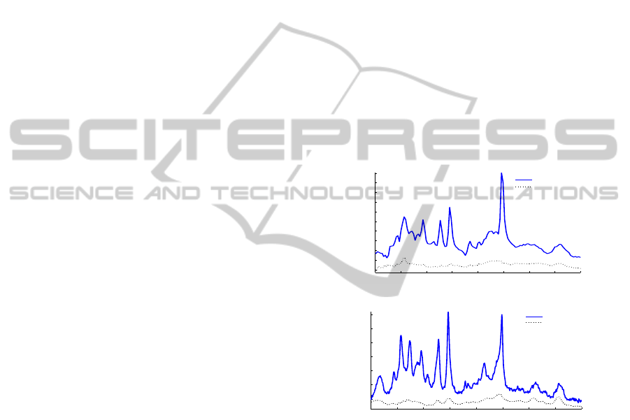
We analyze two types of signals:

• An

H MRS signal from human brain acquired

at 1.5 Tesla (T) on a Philips NT Gyroscan scan-

ner. This signal was obtained using the PRESS

pulse sequence (Bottomley, 1984). MRS parame-

ters were: repetition time of 6s, TE = 23 ms, SW

= 1 KHz and 64 averages. B0 eddy current correc-

tion (Klose, 1990) was performed using the water

reference before quantiﬁcation. See Fig.1 (a).

• An

H MRS signal from rat brain acquired at

9.4 T on a Bruker Biospec small animal MR scan-

ner (Bruker BioSpin MRI, Ettlingen, Germany).

This signal was acquired using the PRESS pulse

sequence (Bottomley, 1984) with implemented

pre-delay Outer Volume Suppression (OVS) and

making use of the water suppression method VA-

POR (Tk´aˇc et al., 1999). MRS parameters were:

repetition time of 8s, TE = 20 ms, SW = 4 KHz

and 128 averages. B0 eddy current correction as

well as B0 drift removalwere performed using the

Bruker built-in routines and shimming was per-

formed using FASTMAP (Gruetter, 1993). See

Fig.1 (b).

Additionally, an unsuppressed water signal is always

measured, which is commonly used as a reference for

phase and lineshape corrections.

0.511.522.533.544.5

0.02

0.04

0.06

0.08

0.1

0.12

0.14

0.16

0.18

0.2

ppm

Amplitude [a.u.]

Signal 1.5T

(a)

0.511.522.533.544.5

x 10

ppm

Amplitude [a.u.]

Signal 9.4T

(b)

Figure 1: Real part of the in vivo spectra. The dotted curve

is the nulled metabolite signal corresponding to the mea-

sured macromolecules and lipids. (a) Human brain signal

acquired at 1.5T. (b) Rat brain signal acquired at 9.4T.

On both scanners, an in vitro basis set of reference

metabolites was measured. The following metabo-

lites were used: Alanine (Ala), Aspartate (Asp), Crea-

tine (Cre), Gamma-Aminoburytic acid (GABA), Glu-

cose (Glc), Glutamine (Gln), Glutamate (Glu), Glyc-

erolphosphorylcholine (GPC), Glutathione (GSH),

Lactate (Lac), Myo-Inositol (m-Ins), N-Acetyl As-

partate (NAA), Phosphorylcholine (PCh), Phospocre-

atine (PCr), Phosphoryl Ethanolamine (PE) and Tau-

rine (Tau). A typical problem for in vivo MRS quan-

tiﬁcation is the presence of a macromolecular sig-

nal affecting the baseline of the spectra. For this

DAMPING FACTOR CONSTRAINTS AND METABOLITE PROFILE SELECTION INFLUENCE MAGNETIC

RESONANCE SPECTROSCOPY DATA QUANTIFICATION

177

study, we measured the in vivo spectrum of macro-

molecules (MM) using an inversion recovery se-

quence. The inversion time was ﬁne-tuned experi-

mentally for metabolite nulling and this MM signal

was added to the basis set of reference metabolites.

3 QUANTIFICATION

3.1 Preprocessing

In in vivo

H MRS signals, the concentration of water

in the brain is several orders of magnitude higher than

the concentration of the metabolites. This signal is

suppressed during acquisition in order to increase the

resolution of the metabolites of interest. Nevertheless,

there is always some residual water around 4.7 ppm

that must be removed to reduce the complexity of the

signal analysis and improve the quantiﬁcation accu-

racy. The signals presented here were ﬁltered using

a method called Hankel Singular Value Decomposi-

tion (Pijnappel et al., 1992), which decomposes the

FID in a sum of exponentials and eliminates the com-

ponents found in the speciﬁc frequency region of the

water. In particular, the more efﬁcient HLSVD-PRO

implementation (Laudadio et al., 2002) is used. Other

preprocessing steps for these signals include phase

correction for better visualization of the spectra, and

time circular shift for the Bruker signals, which were

performed using the jMRUI software package (Stefan

et al., 2009).

3.2 AQSES

The quantiﬁcation method used here for analyzing the

spectra is AQSES (Poullet et al., 2007). This is a time-

domain method that combines metabolite proﬁles in

the best way as expressed in Eq.(1) to ﬁt the signal

under analysis. The most important output parame-

ters of this method are the amplitudes of each metabo-

lite, because these are proportional to the concentra-

tion of metabolites in the tissue. However, the quan-

tiﬁcation method also requires the tunning of other

model parameters such as small frequency shifts f

damping corrections d

and a common phase term

=φ for each metabolite. In particular, the damp-

ing parameters allow the metabolite proﬁles to be nar-

rower or wider for better ﬁtting the signal. An es-

sential model parameter is the upper bound for the

damping parameters used as a constraint in the quan-

tiﬁcation method AQSES. This is needed in order to

avoid metabolite proﬁles to become too broad and

ﬁt the baseline. However, a too low upper bound

is not desired, as metabolites are then badly ﬁtted.

Until now this damping bound was chosen as a ﬁx

value independent on the signal information. In this

study, we propose to estimate this bound as an adap-

tive method that takes into account information from

the signal and the metabolite basis set. To this end, we

make use of the fact that the damping of a complex

damped exponential is equal to the linewidth (i.e. the

Full Width at Half Maximum (FWHM)) of the corre-

sponding Lorentzian peak. Thus, we approximate the

upper bound for the damping factor constraint as the

difference between the FWHM of the unsuppressed

water signal of the in vivo and a singlet from the in

vitro metabolites (i.e. NAA). As can be seen in Fig.1,

there is a macromolecular background signal underly-

ing the in vivo signal. Baseline correction in AQSES

is accounted for by simultaneously using the MM sig-

nal in the basis set as well as a smooth spline model

for additional baseline correction.

3.3 Statistical Residual Analysis

The residual is the difference between the measured

signal and the ﬁt of this signal as obtained by AQSES.

We use the residual in the frequency domain either

for graphical assessment of the goodness-of-ﬁt, or as

an indication of possible ﬁtting problems. If the ﬁt

is correct, the residual should not contain metabolites

and should be white noise. To assess the goodness of

the ﬁt, we use a quality factor proposed by (Slotboom

et al., 2009): Q

fit

(N) =

N.σ

, where σ

is the variance

of the signal noise calculated from the metabolite-free

region, R is the norm of the residual and N is the num-

ber of points of the least-squares ﬁt. This value of Q

fit

is close to 1 when the ﬁt is perfect, bigger than 1 when

the model is probably incomplete (lack of metabo-

lites) and smaller than 1 when parts of the noise are

ﬁtted (overﬁtting) which means that the model has too

many degrees of freedom.

4 RESULTS AND DISCUSSION

4.1 Effect of Damping Factor

Constraint

We study the effect of the damping factor constraint,

which allows each metabolite in the basis set to be as

narrow or wide as the in vivo signal. Figure 2 shows

the results of quantiﬁcation for 3 different damping

factor constraint values. Quantiﬁcation can be ﬁrst

of all evaluated by visual inspection of the residual,

which already provides information about the regions

that are not well-ﬁtted. Setting the upper bound on the

BIOSIGNALS 2011 - International Conference on Bio-inspired Systems and Signal Processing

178

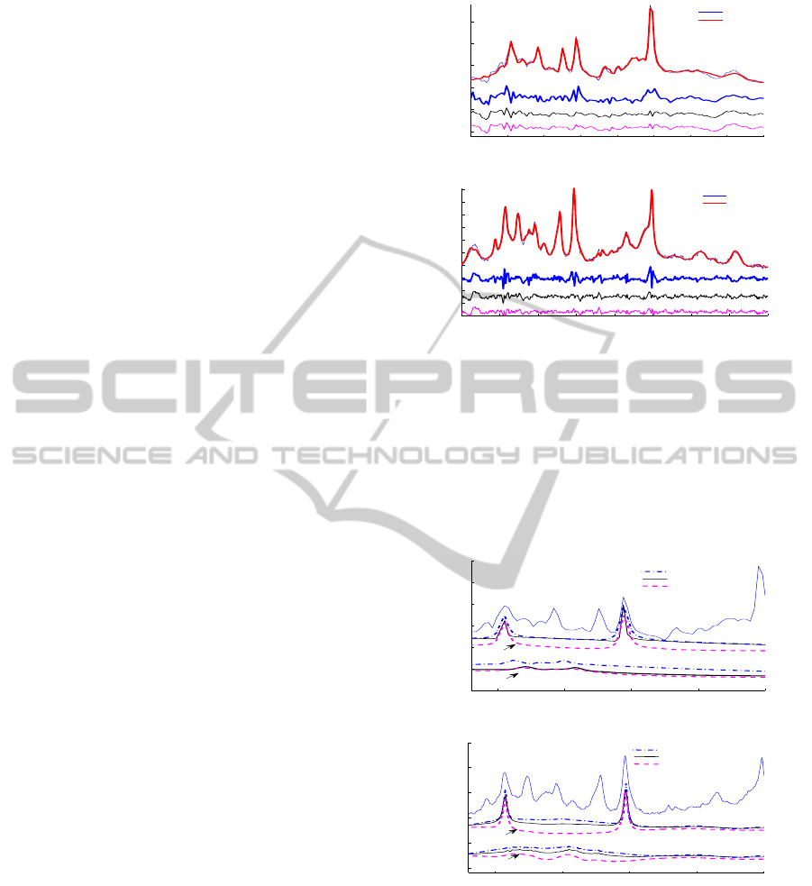
damping factors too low is clearly reﬂected in the pat-

tern of the residual, where peaks with similar shape

are observed in the region of the metabolites. Subse-

quently, when a bigger damping is allowed, improve-

ments in the ﬁtting are reﬂected in the residual (see

Fig.2, e.g. around 2 ppm, 3 ppm and 3.9 ppm). Al-

though large increases of the damping with regards to

the good bound do not improve or worsen the resid-

ual, a more detailed look into the results illustrate that

when a too large damping factor is allowed, some

metabolites may wrongly take over other metabolites

or baseline contribution (see especially the bottom

proﬁle of Glc in Fig.3). Moreover, this effect is not

obvious from the ﬁtting results and it may affect the

stability of the method, leading to wrong estimations.

Correlation is also used to evaluate the goodness

of the ﬁt by correlating the original signal with the ﬁt-

ting. Values close to 1 reﬂect a good correlation and

thus a good ﬁt. However, a good correlation does not

mean good estimates and therefore we must carefully

interpret this parameter. The correlations of the orig-

inal and the ﬁtted signal for the three damping val-

ues at 1.5 T were 0.9234, 0.9770 and 0.9786 respec-

tively; and the correlations for the 9.4 T signal were

0.9241, 0.9808 and 0.9861 respectively. For testing

the assumption that the residual estimated after a good

ﬁt is random noise (i.e. white Gaussian noise), we

evaluated and tested the real and imaginary parts of

the residuals. A zero mean bivariate normal variable

Z = (X,Y) with X andY uncorrelated with equal vari-

ances, σ

= σ

= σ can be expressed in polar coor-

dinates as Z = (Rcos(θ), Rsin(θ)) where the radius

R has a Rayleigh distribution with scale parameter σ

and the angle θ is uniformly distributed on the interval

[−π, π] (Grage and Akke, 2003). This assumption has

been used to assess whether the real and imaginary

parts of the residual are independent and identically

distributed (results not shown here).

4.2 Lack of Metabolites in the Basis Set

Additionally, we study the effect of the number of

metabolites used for quantiﬁcation as this may also

cause over- or underestimation. Fig.4 shows the re-

sults of amplitude estimation for the 1.5 T and 9.4 T

signals when using a complete and incomplete basis

set of metabolites. For the 1.5 T signal we considered

3 groups of metabolite proﬁles: (a) all 13 metabo-

lites (Ala, Asp, Cho, Cre, GABA, Glc, Gln, Glu, Lac,

Myo, NAA, Tau), (b) the 6 most relevant metabolites

having a high concentration in normal brain (Cho,

Cre, Gln, Glu, Myo, NAA), (c) the 4 most relevant

metabolites having the highest concentration (Cho,

Cre, Glu, NAA). For the 9.4 T signal we also con-

0.511.522.533.544.5

−0.1

−0.05

0.05

0.1

0.15

ppm

Amplitude [a.u.]

Signal

Fit

(1) Residual damping 0.001

(2) Residual damping 0.01

(3) Residual damping 0.5

(a)

0.511.522.533.544.5

−8

−6

−4

−2

x 10

ppm

Amplitude [a.u.]

Signal

Fit

(1) Residual damping 0.0025

(2) Residual damping 0.05

(3) Residual damping 0.5

(b)

Figure 2: Quantiﬁcation results using different damping

factor constraints which reﬂect the over- or underestima-

tion of amplitude estimates and the importance of its care-

ful selection. The best ﬁtted signal is the overlapped thick

line and the residuals are the curves beneath. (a) 1.5 T sig-

nal and (b) 9.4 T signal. (1) Residual with damping factor

constraint 0.001 (small bound). (2) Residual with damp-

ing 0.01 factor constraint (good bound). (3) Residual with

damping 0.5 factor constraint (big bound).

22.533.54

−0.1

−0.05

0.05

0.1

0.15

0.2

ppm

Amplitude [a.u.]

Glc

Cre

Small bound

Good bound

Big bound

(a)

22.533.54

−1

−0.5

0.5

1.5

x 10

ppm

Amplitude [a.u.]

Small bound

Glc

Cre

Good bound

Big bound

(b)

Figure 3: Effect of damping factor constraint in metabolites

shows a higher impact in small metabolites. The curves be-

neath the signal correspond to metabolite estimates of Crea-

tine and Glucose using small, good and big damping factor

constraints. (a) 1.5 T signal and (b) 9.4 T signal.

sidered 3 groups of metabolite proﬁles: (a) all 16

metabolites (Ala, Asp, Cre, GABA, GPC, GSH, Glc,

Gln, Glu, Lac, Myo, NAA, PCh, PCr, PE, Tau), (b)

the 8 more relevant metabolites having a high concen-

tration (Cre, GPC, GSH, Gln, Glu, Myo, NAA, PE),

DAMPING FACTOR CONSTRAINTS AND METABOLITE PROFILE SELECTION INFLUENCE MAGNETIC

RESONANCE SPECTROSCOPY DATA QUANTIFICATION

179

Ala Asp Cho Cre GABA Glc Gln Glu Lac Myo NAA Tau

0.5

1.5

Amplitude / Cre

Literature (Provencher)

Estimates 12 Met

Estimates 6 Met

Estimates 4 Met

(a)

Ala Asp Cre GABAGPC GSH Glc Gln Glu Lac Myo NAA PE Tau

0.2

0.4

0.6

0.8

1.2

1.4

1.6

1.8

Amplitude / Cre

Literature (Cudalbu)

Literature (Pfeuffer)

Estimates 16 Met

Estimates 9 Met

Estimates 4 Met

(b)

Figure 4: Amplitude estimates and comparison using a

complete and incomplete basis set. (a) Amplitude estima-

tion of metabolites relative to Cre compared to literature

(Provencher, 2001). (b) Amplitude estimation of metabo-

lites relative to Cre compared to literature (Cudalbu et al.,

2006; Pfeuffer et al., 1999).

00.511.522.533.54

0.02

0.04

0.06

0.08

0.1

0.12

0.14

0.16

0.18

ppm

Amplitude [a.u.]

Signal

Fit

Residual

(a)

ppm

Quality factor (Q)

3.9

3.7

3.5

3.3

3.1

2.9

2.7

2.5

2.3

2.1

1.9

1.7

1.5

1.3

1.1

0.9

0.7

0.5

0.3

0.1

Damp 0.01 − 12 metabolites

Damp 0.01 − 4 metabolites

(b)

Figure 5: Quantiﬁcation analysis via the Quality factor (Q)

for the signal at 1.5 T using an incomplete basis set of

metabolites. (a) Fit using a basis set with 4 metabolites.

(b) Quality factor plot for the signal using a complete and

incomplete basis set (12 and 4 metabolites). The quality

factor computed for the signals was 2.1207 and 7.4472 re-

spectively.

concentration (Cre, GPC, Glu, NAA). Each basis set

is extended with the corresponding MM signal. The

lack of some metabolites in the basis set leads to a

00.511.522.533.54

−2

x 10

ppm

Amplitude [a.u.]

Signal

Fit

Residual

(a)

ppm

Quality factor (Q)

0.1

0.3

0.5

0.7

0.9

1.1

1.3

1.5

1.7

1.9

2.1

2.3

2.5

2.7

2.9

3.1

3.3

3.5

3.7

3.9

Damp 0.05 − 12 metabolites

Damp 0.05 − 4 metabolites

(b)

Figure 6: Quantiﬁcation analysis via the Quality factor (Q)

for the signal at 9.4 T using an incomplete basis set of

metabolites. (a) Fit using a basis set with 4 metabolites.

(b) Quality factor plot for the signal using a complete and

incomplete basis set (16 and 4 metabolites). The quality

factor computed for the signals was 1.4033 and 5.1740 re-

spectively.

slight under- or overestimation of some other metabo-

lites and this is also reﬂected in the residual. Ampli-

tude estimates in Fig.4 are close to those presented

in literature, however, it is important to mention that

they are highly affected by individual conditions of

the tissues, small differences in the measurement pa-

rameters, size of the voxel measured and therefore di-

verse concentration ranges are found in similar stud-

ies, leading to a high variability of the amplitude es-

timates. In Fig.5 (a) and 6 (a) we observe that the

ﬁts with an incomplete basis set are not good and the

corresponding Q

fit

of 7.4472 and 5.1740 also conﬁrm

the imperfect quantiﬁcation. In order to further eval-

uate the quantiﬁcation, we selected a span or window

of 0.1 ppm to evaluate the quality factor in a moving

window. In Fig.5 (b) and 6 (b) we present the results

of this quality measure where the plotted curves rep-

resent the Q

fit

values obtained for all the frequency

intervals selected and the dashed line represents the

conﬁdence bound calculated as three times the stan-

dard deviation (

> (3σ)

or equivalently Q

fit

> 9).

A missing metabolite is considered when the Q

fit

value is higher than the selected threshold.

5 CONCLUSIONS

Reliable metabolite estimation of in vivo MRS sig-

nals for determination of metabolite concentrations is

of paramount importance for obtaining additional in-

formation in the diagnostics of cancer and metabolic

BIOSIGNALS 2011 - International Conference on Bio-inspired Systems and Signal Processing

180

diseases. Therefore, quantiﬁcation of MRS signals

was performed evaluating the inﬂuence of the damp-

ing factor constraint and the number of components

used in the metabolite basis set used for quantiﬁca-

tion. We observed in particular, that the damping fac-

tor in the quantiﬁcation method AQSES plays an im-

portant role in amplitude estimation. From the quan-

tiﬁcation results, we examined the residual and ana-

lyzed the ﬁt of the individual components which are

sensible to quantiﬁcation constraints. The selection of

the metabolites for the basis set is important for quan-

tiﬁcation, thus an incomplete basis set will provide ﬁts

where one metabolite ﬁts the region that corresponds

to its neighbor. The residual is used to determine the

goodness of the estimates. It is assumed that a good

estimate will lead to residuals resembling pure white

noise. A test of normality would also help to analyze

the residual and determine how close it is to white

noise.

ACKNOWLEDGEMENTS

Maria I. Osorio Garcia and Dr. Flemming U. Nielsen

are Marie Curie research fellows in the EU train-

ing network FAST (www.fast-mrs.eu). Dr. Diana M.

Sima is a postdoctoral fellow of the Fund for Sci-

entiﬁc Research-Flanders. Prof. Dr. Uwe Himmelre-

ich and Prof. Dr. ir Sabine Van Huffel are full pro-

fessors at the Katholieke Universiteit Leuven, Bel-

gium. Research supported by: Research Council

KUL: GOA Ambiorics, GOA MaNet, CoE EF/05/006

Optimization in Engineering (OPTEC), IDO 05/010

EEG-fMRI, IDO 08/013 Autism, IOF-KP06/11 Fun-

Copt, several PhD/postdoc & fellow grants; Flem-

ish Government: FWO: PhD/postdoc grants, projects:

FWO G.0302.07 (SVM), G.0341.07 (Data fusion),

G.0427.10N (Integrated EEG-fMRI) research com-

munities (ICCoS, ANMMM); IWT: TBM070713-

Accelero, TBM070706-IOTA3, TBM080658-MRI

(EEG-fMRI), PhD Grants; Belgian Federal Science

Policy Ofﬁce: IUAP P6/04 (DYSCO, ‘Dynami-

cal systems, control and optimization’, 2007-2011);

ESA PRODEX No 90348 (sleep homeostasis), EU:

FAST (FP6-MC-RTN-035801), Neuromath (COST-

BM0601), KU Leuven center of Excellence ’MO-

SAIC’.

REFERENCES

Bottomley, P. (1984). Selective volume method for perform-

ing localized NMR spectroscopy. in U.S patent, (4 480

228).

Cudalbu, C., Cavassila, S., Ratiney, H., Grenier, D.,

Briguet, A., and Graveron-Demilly, D. (2006). Esti-

mation of metabolite concentrations of healthy mouse

brain by magnetic resonance spectroscopy at 7T.

Comptes Rendus Chimie, 9(3-4):534 – 538.

Grage, H. and Akke, M. (2003). A statistical analysis of

NMR spectrometer noise. Journal of Magnetic Reso-

nance, 162(1):176 – 188.

Gruetter, R. (1993). Automatic localized in vivo adjustment

of all ﬁrst- and second- order shim coils. Magnetic

Resonance in Medicine, 29(6):804–811.

Klose, U. (1990). In vivo proton spectroscopy in presence

of eddy currents. Magnetic Resonance in Medicine,

14(1):26 – 30.

Laudadio, T., Mastronardi, N., Vanhamme, L., Van Hecke,

P., and Van Huffel, S. (2002). Improved Lanczos algo-

rithms for blackbox MRS data quantitation. Jorunal

of Magnetic Resonance, 157(2):292 – 297.

Pfeuffer, J., Tkc, I., Provencher, S. W., and Gruetter, R.

(1999). Toward an in vivo neurochemical proﬁle:

Quantiﬁcation of 18 metabolites in short-echo-time

H NMR spectra of the rat brain. Journal of Magnetic

Resonance, 141(1):104 – 120.

Pijnappel, W. W. F., van den Boogaart, A., de Beer, R., and

van Ormondt, D. (1992). SVD-based quantiﬁcation

of magnetic resonance signals. Journal of Magnetic

Resonance, 97(1):122 – 134.

Poullet, J.-B., Sima, D., Simonetti, A., De Neuter, B.,

Vanhamme, L., Lemmerling, P., and Van Huffel, S.

(2007). An automated quantitation of short echo time

MRS spectra in an open source software environment:

AQSES. NMR in Biomedicine, 20(5):493 – 504.

Provencher, S. (2001). Automatic quantitation of local-

ized in vivo

H spectra with LCModel. NMR in

Biomedicine, 14(4):260–264.

Ratiney, H., Coenradie, Y., Cavassila, S., van Ormondt,

D., and Graveron-Demilly, D. (2004). Time-domain

quantitation of

H short echo-time signals: back-

ground accommodation. MAGMA, 16(6):284 – 296.

Slotboom, J., Nirkko, A., Brekenfeld, C., and van Ordmont,

D. (2009). Reliability testing of in vivo magnetic reso-

nance spectroscopy (MRS) signals and signal artifact

reduction by order statistics ﬁltering. Measurement

Science and Technology, 20(104030):14pp.

Stefan, D., Di Cesare, F., Andrasescu, A., Popa, E.,

Lazariev, A., Vescovo, E., Strbak, O., Williams, S.,

Starcuk, Z., Cabanas, M., van Ormondt, D., and

Graveron-Demilly., D. (2009). Quantitation of mag-

netic resonance spectroscopy signals: the jMRUI soft-

ware package. Measurement Science and Technology,

20(10):104035(9pp).

Tk´aˇc, I., Starˇcuk, Z., Choi, I.-Y., and Gruetter, R. (1999). In

vivo

H NMR spectroscopy of rat brain at 1ms echo

time. Magnetic Resonance in Medicine, 41(4):649–

656.

DAMPING FACTOR CONSTRAINTS AND METABOLITE PROFILE SELECTION INFLUENCE MAGNETIC

RESONANCE SPECTROSCOPY DATA QUANTIFICATION

181