AN ADAPTIVE INTERFACE FOR ACTIVE LOCALIZATION

Kenji Okuma, Eric Brochu, David G. Lowe and James J. Little

The University of British Columbia, Vancouver, Canada

Keywords:

Object localization, Active learning, Adaptive interface.

Abstract:

Thanks to large-scale image repositories, vast amounts of data for object recognition are now easily available.

However, acquiring training labels for arbitrary objects still requires tedious and expensive human effort. This

is particularly true for localization, where humans must not only provide labels, but also training windows

in an image. We present an approach for reducing the number of labelled training instances required to

train an object classiﬁer and for assisting the user in specifying optimal object location windows. As part

of this process, the algorithm performs localization to ﬁnd bounding windows for training examples that are

best aligned with the current classiﬁcation function, which optimizes learning and reduces human effort. To

test this approach, we introduce an active learning extension to a latent SVM learning algorithm. Our user

interface for training object detectors employs real-time interaction with a human user. Our active learning

system provides a mean performance improvement of 4.5% in the average precision over a state of the art

detector on the PASCAL Visual Object Classes Challenge 2007 with an average of just 40 minutes of human

labelling effort per class.

1 INTRODUCTION

It is possible to improve the classiﬁcation perfor-

mance of machine learning methods for object recog-

nition by simply providing more training examples.

However, the cost of providing labelled data—asking

a human to examine images and provide labels—

becomes impractical as training sets grow.

In addition, object localization with bounding

windows is important for many applications and plays

a signiﬁcant role in improved performance (Lazebnik

et al., 2006; Mutch and Lowe, 2006; Viola and Jones,

2004), but this also places an increased burden on hu-

man labelling by requiring accurately aligned bound-

ing windows around each training instance.

We present a method for using active learning

(Settles, 2010; Tong and Koller, 2001) to reduce

the required number of labelled training examples to

achieve a given level of performance. Our method

also proposes optimal bounding windows aligned

with the current classiﬁcation function. Active learn-

ing refers to any situation in which the learning algo-

rithm has control over the inputs on which it trains,

querying an oracle to provide labels for selected im-

ages. In particular, we are concerned with the prob-

lem where a person is required to provide labels

for bounding windows. Unlike image classiﬁcation

where the image is classiﬁed as a whole, we apply this

approach to object localization by iteratively select-

ing the most uncertain unlabelled training windows

from a large pool of windows, and present them to

the user for labelling. If the object of interest is cor-

rectly bounded by the localization window, the hu-

man provides a positive label, otherwise they provide

a negative label or indicate their uncertainty. We have

designed a user interface that is efﬁcient for the user

and provides feedback on performance while also en-

abling the user to retain some initiative in selecting

image windows.

Our experimental results apply the approach to

the PASCAL Visual Object Classes 2007 (VOC2007)

(Everingham et al., 2007) on twenty different cat-

egories learned with mixtures of multi-scale de-

formable part models from Felzenswalb et al.

(Felzenszwalb et al., 2009), one of two joint win-

ners in the VOC2009 challenge for object localization

problems. In the ﬁrst experiment, we show that we

can match their results on VOC2007 data while using

many fewer labelled windows for training. Then we

demonstrate our full user interface on more diverse

images, such as those obtained from web search en-

gines and show how it enables a user to efﬁciently

improve performance on VOC2007. While these ex-

periments show that our actively trained deformable

part model works well with active learning, the sys-

tem does not depend on a speciﬁc classiﬁer or fea-

248

Okuma K., Brochu E., G. Lowe D. and J. Little J..

AN ADAPTIVE INTERFACE FOR ACTIVE LOCALIZATION.

DOI: 10.5220/0003317302480258

In Proceedings of the International Conference on Computer Vision Theory and Applications (VISAPP-2011), pages 248-258

ISBN: 978-989-8425-47-8

 2011 SCITEPRESS (Science and Technology Publications, Lda.)

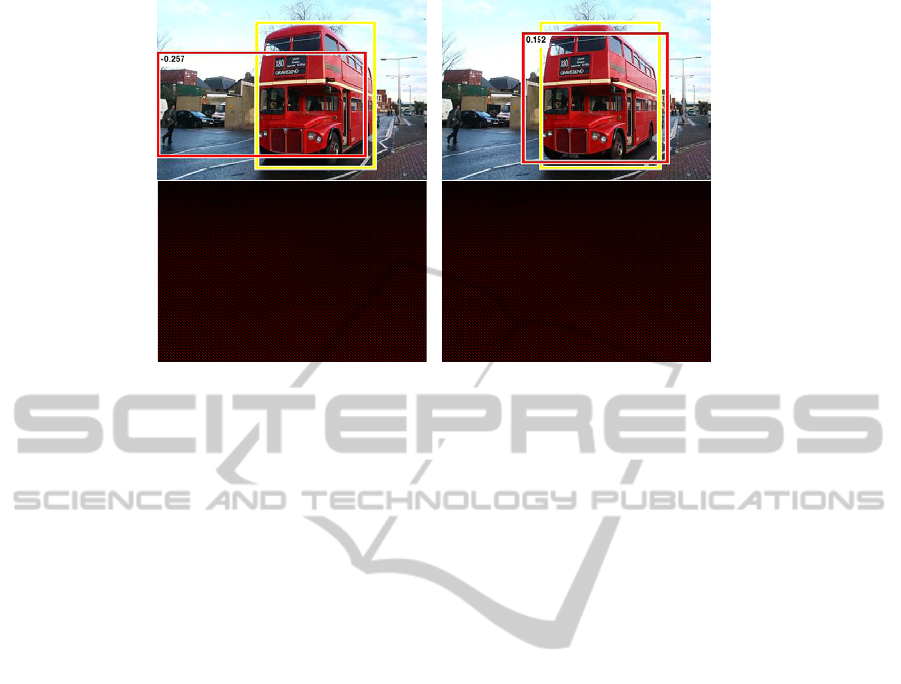
Figure 1: Screen shots of object detection results. This shows how our active learning approach improves object local-

ization. The top left shows the highest scoring detection using only VOC 2007 data, whereas the top right shows the result

after retraining with additional data obtained using our active learning interface. The bottom row shows associated conﬁdence

maps in the same scale. Note how the detection conﬁdence increased and the peak position was shifted. Yellow boxes are the

ground truth and red boxes are detections with the associated detection conﬁdence.

ture set. If other classiﬁers or features are found to

be more suitable to a domain, we can also incorporate

them into our framework.

2 ACTIVE LEARNING FOR

IMAGE LABELLING

Image labelling requires human effort to supply the

labels for each positive window in the training set.

This typically involves thousands of instances, and

is thus extremely labour-intensive. To make object

recognition practical over multiple domains, we need

to recognize that human labelling is a costly resource,

and must be used as efﬁciently as possible. Ac-

tive learning is the machine learning method typically

used in this case. A full discussion of active learning

is beyond the scope of this paper, so we will focus

only on the most relevant areas for our work. We di-

rect the interested reader to, e.g., the recent review by

Settles (Settles, 2010) for a more extensive survey.

In pool-based active learning, which we use here,

candidate data are selectively sampled for labelling

from a pool of unlabelled data U. The model is

then updated to take the new labels into account,

and new candidates selected. Candidate selection

is typically performed by greedily selecting data x

∗

from U according to some utility function, x

∗

argmax

x∈U

U(x). The process repeats as long as the

human labeller is willing, or until some other termi-

nation condition is reached.

The candidate selection objective function is de-

signed to maximize the utility of the labels gathered,

typically by some measure of the expected informa-

tiveness of the labels. This is what makes active learn-

ing efﬁcient in situations where data is plentiful but

labelling it is expensive. By identifying the training

instances that actually impact the model, fewer la-

bels are required, and the bottleneck can be reduced.

In Section 3.1, we use an uncertainty sampling util-

ity function (Lewis and Gale, 1994), which is popu-

lar as it performs well on a variety of problems and

has been extensively studied. Other methods include

maximizing entropy, combining a committee of mod-

els, or maximizing the expected model change.

In recent years, active learning in computer vi-

sion has gained much attention. While various active

learning extensions have been proposed in image clas-

siﬁcation (Collins et al., 2008; Kapoor et al., 2007;

Qi et al., 2008; Vijayanarasimhan et al., 2010; Zhang

et al., 2008), relatively little attention has been paid to

the more challenging problem of object localization

(Abramson and Freund, 2005; Siddiquie and Gupta,

2010; Vijayanarasimhan and Kapoor, 2010). Object

localization requires a model that can identify bound-

ing windows for the object in each image—there can

be zero, one or many such boxes in a single im-

age. Image classiﬁcation needs to consider only a sin-

gle global classiﬁcation per image. Applying active

learning to localization requires a substantial change

in approach, as a single label cannot be applied to an

image—it much be applied to potentially numerous

and overlapping windows of an image. Most active

learning approaches are therefore infeasible for ob-

AN ADAPTIVE INTERFACE FOR ACTIVE LOCALIZATION

249

ject localization problems in even a relatively large

scale dataset such as the VOC2007 dataset of around

10,000 images. To the best of our knowledge, we are

the ﬁrst to apply and test active learning performance

on the PASCAL or similar datasets.

3 ALGORITHM

Our system for active learning uses the Support Vec-

tor Machine (SVM) (Sch

olkopf and Smola, 2002)

classiﬁer, which has proven its success in many state-

of-the-art recognition systems (Dalal and Triggs,

2005; Moosmann et al., 2006; Mutch and Lowe,

2006; Zhang et al., 2006). We also incorporate the re-

cent latent SVM (LSVM) approach of Felzenszwalb

et al. (Felzenszwalb et al., 2009). We will brieﬂy

review these models and describe how we incorpo-

rate active learning. The goal of a supervised learning

algorithm is to take n training samples and design a

classiﬁer that is capable of distinguishing M different

classes. For a given training set (x

, y

), . . . , (x

, y

)

with x

∈ ℜ

and y

∈ −1, +1 in their simplest form

with two classes, LSVM is a classiﬁer that scores a

sample x with the following function (Felzenszwalb

et al., 2009),

(x) = max

z∈Z(x)

β · Φ(x, z) (1)

Here β is a vector of model parameters and z are latent

values. The set Z(x) deﬁnes possible latent values for

a sample x. Training β then becomes the following

optimization problem.

min

β,ξ

≥0

∑

i=1

(2)

s.t. ∀i ∈ {1, . . . , n} : y

) + b ≥ 1 − ξ

(3)

and ξ

≥ 0 (4)

where C controls the tradeoff between regularization

and constraint violation. For obtaining a binary la-

bel for x, we have the decision function, sign(h(x)),

where

h(x) = f

(x) + b (5)

In general, a latent SVM is a non-convex optimiza-

tion problem. However, by considering a single pos-

sible latent value for each positive sample that can be

speciﬁed in training, it becomes a convex optimiza-

tion problem for classical SVMs. For multi-scale de-

formable part models, the set of latent values repre-

sents the location of parts for the object.

3.1 Active Learning on a Latent SVM

We incorporate active learning into an LSVM by at

each iteration selecting the candidate that has the min-

imum distance to the decision boundary. That is, for

a set of data C ⊆ U, where U is the set of unlabelled

image windows, we select:

argmin

x∈C



h(x

)



(6)

This is the candidate datum we ask the human expert

to label. Ideally, we then move the new labelled da-

tum from the candidate to the training set, update the

LSVM model, and repeat, selecting a new candidate

based on the updated model. However, due to the

heavy computational load of LSVM, we choose to up-

date the model in a batch after collecting a set of new

labelled data. In our experiments, we obtain a set of

unlabelled image windows by applying a sliding win-

dow at multiple scales on the image and computing

a Histogram of Oriented Gradients (HOG) descriptor

(Dalal and Triggs, 2005; Felzenszwalb et al., 2009)

from each window as our datum.

This uncertainty sampling utility seeks to label

the most uncertain unlabelled datum to maximize the

margin. There are known to be other successful cri-

teria for SVM active learning, particularly version

space methods (Tong and Koller, 2001). We use un-

certainty sampling as we wish to remain agnostic as

to the underlying model. It has also been shown to

perform well and has the advantage of being fast to

compute and easy to implement. The learning task

then becomes an iterative training process as is shown

in Algorithm 1.

4 EXPERIMENTS

We will ﬁrst test our active learning approach against

a state-of-the-art object detector on VOC2007 (Ever-

ingham et al., 2007) to show the ability to reduce la-

belling requirements without sacriﬁcing performance

. Then we will describe our user interface for active

learning and show its effective performance over the

object categories of the VOC2007 dataset.

4.1 The PASCAL Visual Object Classes

2007

The PASCAL Visual Challenge has been known as

one of the most challenging testbeds in object recog-

nition. The VOC2007 dataset contains 9,963 images:

50% are used for training/validation and the other

VISAPP 2011 - International Conference on Computer Vision Theory and Applications

250

Algorithm 1: Pool-based active learning algorithm for im-

age window labelling

x is a window descriptor, I is a set of m images, L

is a set of labelled image windows and U is a set of

unlabelled windows.

1: {Collect a set of unlabelled image windows, U}

2: U =

3: for i ∈ I do

4: U = U ∪ x where x is the highest scoring de-

tection window in image i

5: end for

6: while the user continues the active learning ses-

sion do

7: {Obtain a set of new labelled data, C , Y }

8: C =

9: Y =

10: for t = 1 to n do

11: x

∗

= argmin

x∈U



h(x

)



12: Get the label y

∗

of the datum x

∗

from the

human expert

13: The expert can add a set of k samples X =

, x

, · ·· , x

} in case of miss detections or

false positives with a set of associated labels

L = {y

, y

, · ·· , y

} of X

14: C = C ∪ x

∗

∪ X

15: Y = Y ∪ y

∗

∪ L

16: U = U − x

∗

17: end for

18: Add C and Y to the training set and update the

LSVM model,

β, { ˆx

, ˆz

}

l=1

and

b where m is

the number of support vectors

19: end while

50% are used for testing. We used VOC2007 to

test our active learning approach to see if it would re-

duce labelling requirements for positive data. We use

our own Python implementation of Felzenszwalb et

al.’s detector (Felzenszwalb et al., 2009) with multi-

scale deformable part models. The original source

code is available online and written in Matlab and C

In our ﬁrst experiment, we used the data provided

by the VOC2007 dataset to show that active learning

could achieve the same classiﬁcation performance by

using only an actively selected subset of the data. To

show the reduced data requirements for active learn-

ing, we trained our model in each category on four

different positive datasets, including 25%, 50%, 75%

and 100% of all positive training images, comparing

the effect of adding training data randomly and ac-

tively. We used the same negative dataset in these ex-

periments, as negative data is cheap to collect. For

The source code is publicly available at

http://people.cs.uchicago.edu/∼pff/latent/

both the random and active data sets, we start by

randomly selecting the ﬁrst 25% of positive images

and training. In the random training set, we then

repeatedly add a further 25% of the positive images

and train again, until all the available data have been

added. We performed active sampling by ﬁrst train-

ing our base model with a randomly selected 25% of

the positive data. We used the base model to choose

the most uncertain positive images from the remain-

ing pool of positive data, repeatedly adding 25% of

the data. Due to randomness in the training procedure,

we repeated these experiments ﬁve times and present

average results with error bars. Figure 2 shows the

results of all twenty categories.

This simulation shows that active sampling is ef-

fective at selecting the most useful data for training.

In most cases, a total of only half of all positive data

is required to get the performance of the full training

set.

5 APPLICATION

In this section, we introduce the active localization

interface for our interactive labelling system, ALOR

(Active Learning for Object Recognition). Our inter-

face iteratively presents the most informative query

windows to the user and allows the user to correct

mistakes made by the model. It is designed to work

on any arbitrary user speciﬁed object category, using

web images it automatically collects from major web

search engines such as Google, Yahoo, and Flickr.

Here, we demonstrate the interface on the “cow” cate-

gory by using a set of images from the Google Image

search engine.

We ﬁrst collect a set of images from the Google

Image search engine with query keywords such as

“cow.” We then use our cow detector that is trained

with VOC2007 data as shown in Figure 2 and let the

algorithm actively select each query. Figure 3 shows

some screen shots of our system interface, which de-

scribes four major cases for labelling data. These

cases are: (a) the window is indeed a cow, (b) the

window is not a cow, (c) the window is ambiguous,

perhaps due to partial overlap, so the window should

be ignored for training, and ﬁnally (d) a user wishes

to add a positive instance that was missed by the clas-

siﬁer or correct false positives. The rectangular boxes

(in red) are queries selected by active learning with

the minimum distance to the decision boundary. The

green boxes are positive classiﬁcations in the current

image that were not selected as queries. These green

boxes are useful for giving the user feedback on the

current classiﬁer performance and to allow the addi-

AN ADAPTIVE INTERFACE FOR ACTIVE LOCALIZATION

251

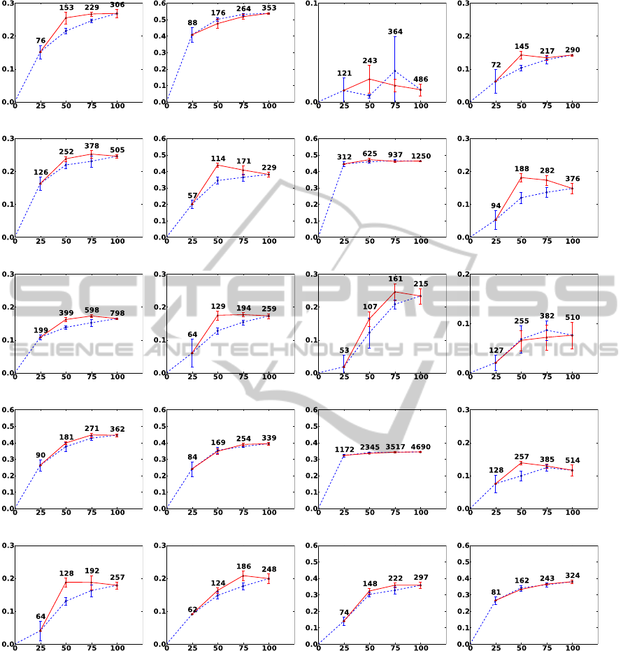
(a) aeroplane (.268) (b) bicycle (.537) (c) bird (.009) (d) boat (.142)

(e) bottle (.245) (f) bus (.376) (g) car (.463) (h) cat (.143)

(i) chair (.163) (j) cow (.173) (k) table (.233) (l) dog (.061)

(m) horse (.443) (n) motorbike (.393) (o) person (.344) (p) plant (.117)

(q) sheep (.179) (r) sofa (.196) (s) train (.355) (t) tvmonitor (.380)

Figure 2: VOC2007: Random vs. active sampling of positive data. There are 20 different visual categories. The horizontal

axis of each ﬁgure represents the portion of positive training samples in percent (%) and the vertical axis gives the average

precision. The solid red line shows the result of active sampling and the dotted blue line is for random sampling. We performed

both random and active sampling of positive data ﬁve times with a different random seed. The errorbars are based on one

standard deviation. For both random and active data sets, we start by training on a randomly selected 25% of positive samples.

In the random training set, we then repeatedly add a further 25% of the positive samples and train again. In the active set, we

added an additional 25% of actively selected samples iteratively until we use the full positive data. The number of positive

samples in each subset is shown above each errorbar. The ﬁnal average precision with the full positive data is shown next to

the name of a category. Note that the result of active sampling often performs better with 50 % or 75 % of the images.

VISAPP 2011 - International Conference on Computer Vision Theory and Applications

252

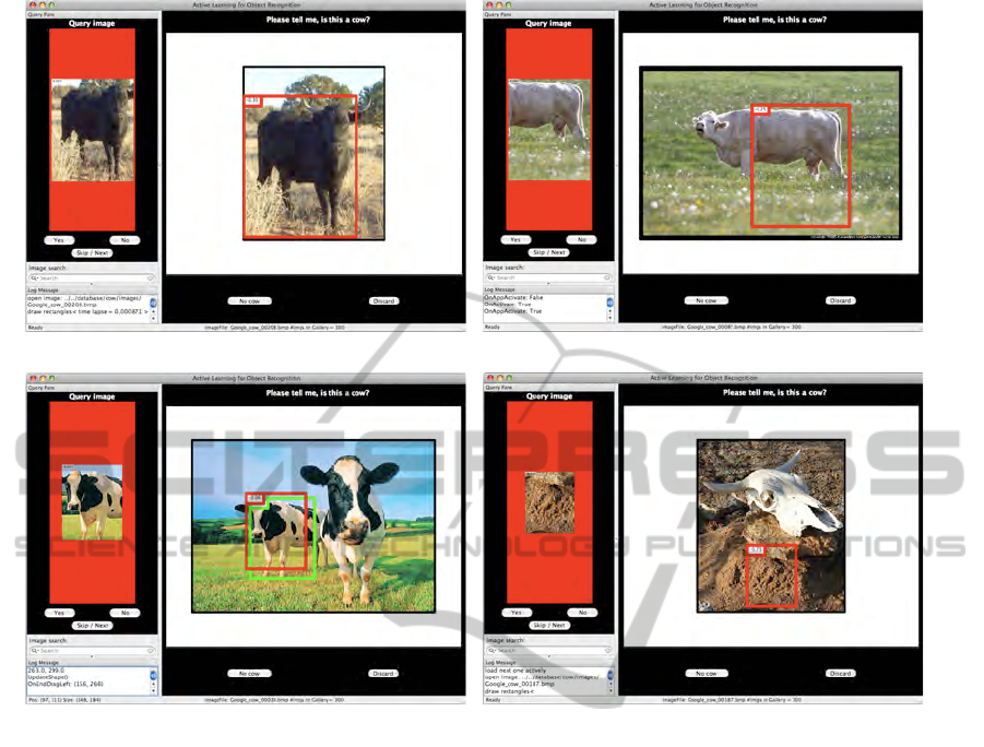
(a) Case 1: YES (b) Case 2: NO

Figure 3: Screen shots of our interactive labelling system with our actively tranined LSVM. This ﬁgure shows a set of

screen shots of our interactive labelling system. In each case, the query window to be labelled is shown on the left, and the

image from which it was selected is shown on the right (with the query window highlighted in red). (a) shows an instance

when the query window is indeed a cow, so the appropriate answer is YES. (b) shows an example bounding window that is

not a cow, so the answer is NO. Note that the bounding window partially covers a real cow, so it would not be obtained from

the usual approach of labelling negative images. (c) shows a query window where it is hard to decide whether it is a cow, due

to being largely occluded, misplaced, or incorporating multiple cows, so the answer is MAYBE, in which case we can just

skip the query. (d) shows an instance in which an image does not contain any cow. In such case, a human user can specify

that all windows in the image are negative examples and a machine selects only false positive windows. In the case of missed

detections, a human user can specify the centroid of the object by clicking on the image and the current classiﬁer suggests the

optimally aligned bounding window with the highest classiﬁcation conﬁdence.

tion of rare training examples that may lie far enough

away from the decision boundary that they may oth-

erwise never be detected or queried.

When a user wishes to add a training example that

was not queried, they can simply click on the image.

This will select the window with the highest classi-

ﬁcation conﬁdence that contains the location of the

mouse click. Therefore, the current classiﬁer is still

used to select the best-aligned training window, and

user effort is minimized.

The interface is written in Python and C and uti-

lizes multi-core CPUs to speed up the process and re-

alize real-time interactions between a human user and

a machine. Our interface currently takes less than a

second (on an 8-core machine) to update and deter-

mine the next query windows upon receiving new la-

bels, though the precise time depends on the number

of dimensions of visual features and the resolution of

the image. The interactive process can be sped up by

precomputing image features, which we did in our ex-

periments shown in Table 1.

5.1 The PASCAL Visual Object Classes

In this section, we demonstrate that our prototype

active learning GUI enables fast, efﬁcient labelling

AN ADAPTIVE INTERFACE FOR ACTIVE LOCALIZATION

253

BICYCLE (.537)

TOP 5:

WORST 5:

SOFA (.257)

TOP 5:

WORST 5:

CHAIR (.163)

TOP 5:

WORST 5:

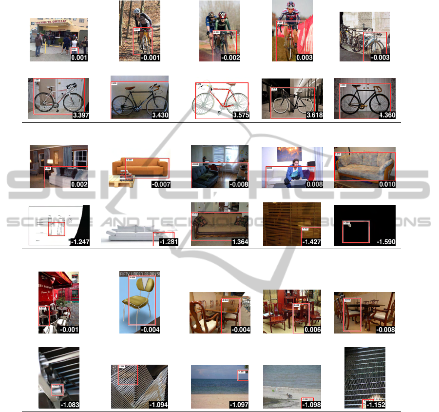
Figure 4: Training images from Flickr, sorted for active learning. This shows query windows for three categories. For

each category, the best 5 and worst 5 actively selected query windows are shown. For each category, we downloaded 3,000

images from the Flickr image search with keywords such as “bicycle”, “sofa”, and “chair.” These web images are then

sorted based on the window with the highest classiﬁcation conﬁdence in each image, as described in Algorithm 1 in Section

3.1. The red box represents the query window for the image with the associated detection score shown at the bottom right

corner of the image. Large positive scores indicate high conﬁdence that the object is present, large magnitude negative scores

indicate conﬁdence that it is not present, while scores near zero represent maximum uncertainty (are close to the margin). The

categories are ordered with the average precision shown next to the category title. Note that the worst 5 query windows in the

bicycle category contain target objects that are easily classiﬁed, whereas the worst 5 query windows in the chair category do

not contain any target objects. In the sofa category with the middle AP score, the worst 5 query windows include ones that

contain target objects and ones without.

to improve performance on data from the PASCAL

VOC2007. For comparison, we ﬁrst prepare our base-

line detectors by training a latent SVM with HOG on

all twenty categories. The third column of Table 1

shows the average precision of each category. Due

to randomness in the training procedure, those num-

bers do not exactly match with ones in (Felzenszwalb

et al., 2009) even with the same parameter settings,

VISAPP 2011 - International Conference on Computer Vision Theory and Applications

254

but they differ by less than 1 percent.

Next we perform a pool-based active learning ses-

sion using Algorithm 1 with our active learning GUI

to train these baseline detectors and improve their per-

formance. With our interface, we collect training im-

ages from Flickr, which was a source for VOC2007

images. We used the Flickr Image API to obtain only

images from after the competition date of VOC2007

to prevent the possibility of obtaining test data from

the competition. Our interface allows a human user to

search images based on a query word such as “cow,”

“motorbike,” etc. We collected the ﬁrst 3000 images

from the Flickr database in each category. In order to

further speed up the training process, we also cache

visual features, using our baseline detectors to scan

images, and sort them based on the uncertainty score

in Eq. (6) for the highest detection scoring window.

It takes approximately 3-4 hours to search, download

and scan 3000 images (around 164 million bounding

windows) to generate the set of most-uncertain query

windows. However, this preprocessing can be done

with no human interaction other than specifying the

tag. The effectiveness of active learning can be seen

in Figure 4 which shows the best 5 and worst 5 ac-

tively selected query windows in each category. The

worst 5 query windows in the bicycle category con-

tain target objects that are easily classiﬁed, whereas

the worst 5 query windows in the chair category do

not contain any target objects. In the sofa category,

the worst 5 query windows include ones that contain

easy target objects as well as ones without.

Table 1 summarizes the results and training data

statistics. We downloaded in total 60,000 images

from Flickr and annotated bounding windows in 300

actively selected images for each category based on

uncertainty of the highest scoring detection window

of each image. We used the highest scoring detection

window for sorting images in order to get as many

positive labels as possible from a large unlabelled

data pool. We then conducted two simulations. One

is a common active learning approach where we an-

swer just 300 query windows based on our uncertainty

sampling criteria (ALORquery). The other is a case

of fully utilizing our interface where we are allowed

to not only answer these 300 query windows but also

add user selected query windows (ALORfull). The

time required for the human interactive labelling of

these 300 image queries was around 20 minutes and

less than 40 minutes was required for fully utilizing

our interface and giving more annotations for each

category.

Figure 5 shows the performance comparison of

both ALORquery and ALORfull in a different num-

ber of training images. It shows that ALORfull con-

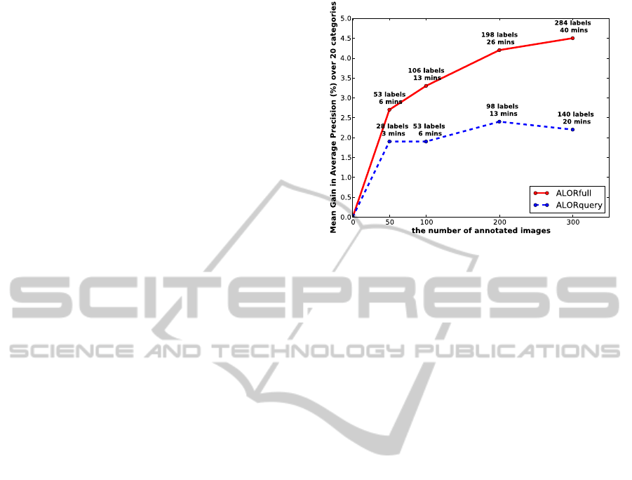
Figure 5: Performance comparison of ALORfull and

ALORquery. Each point represents the average number of

additional positive labels and the average training time per

category. By allowing a user to add additional queries, the

performance is consistently better. Note that just 53 labels

from ALORfull outperform 140 labels from ALORquery.

sistently outperforms ALORquery, which indicates

that user selected queries improve the overall detec-

tion performance. More results in Table 2 demon-

strate an impact of user selected queries on the ﬁnal

classiﬁcation performance. In the table, we show the

result of ALORquery with 300 images and ALORfull

with 100 and 300 images. For the cases of ALOR-

full, around 40 % of queries are selected by a user.

Those queries are often quite challenging for a ma-

chine to choose, because they are often either erro-

neous or missed detections and distant from the de-

cision boundary of a latent SVM. A human oracle is

quite helpful in such cases.

Fig. 6 presents the gain of our best result for each

category in the average precision. From our exper-

iments, we can make several observations. First, in

most of the categories, our active learning interface

allows a user to quickly improve the performance of

the baseline detectors. Second, our user interface also

allows a user to achieve a better performance than

would be obtained by a simpler learning approach in

which a user answers Yes/No/Maybe queries for se-

lected windows. A lot of difﬁcult machine-selected

queries that a user is not sure about (Fig. 3(c), for

example) can be easily corrected with our interface.

Third, with less than 40 minutes of user input, we can

achieve signiﬁcant performance improvement even

over the best competition results. The PASCAL com-

petition has a section in which users can provide their

own data, but the difﬁculty of collecting such data

means there have seldom been entries in that section.

Our active learning approach and GUI would enable

users to efﬁciently collect useful data for improved

AN ADAPTIVE INTERFACE FOR ACTIVE LOCALIZATION

255

Table 1: Average precision on VOC2007 and training data statistics. This ﬁgure shows the result of our experiments and

training data statistics. The ﬁrst section shows the number of object labels in VOC2007 data and the result obtained by our

implementation of the baseline latent-SVM with HOG (Felzenszwalb et al., 2009) on VOC2007 test data (i.e., LSVM+HOG).

The middle section shows the total number of additional positive and negative labels and the AP score with these additional

labels. We obtained the additional data by using models from LSVM+HOG and our active learning GUI on only 300 actively

selected images (one query per image, 300 queries in total) out of 3000 web images for each category. This represents a

common active learning approach with uncertainty sampling criteria where a user is not allowed to add any additional queries

and is only queried by a machine (i.e., ALORquery). The last section shows additional labels and AP scores on the same

300 actively selected images. But a user is now allowed to fully utilize our interface by not only answering queries from

a machine but also adding his/her own queries with our interface (i.e., ALORfull). It required only about 20 minutes per

class for a person using our interface to improve the results from the ﬁrst column and takes about 40 minutes to get the best

performance improvement shown in the third column. Note that a user selects roughly 100 ∼ 200 additional query windows

in each category, which are mostly erroneous or missed detections that are never selected by the uncertainty criteria, but

effectively presented by our interface. The best AP scores are in bold face and these best scores already exceed the best

competition results (of any method) over 17 of 20 categories from VOC2007 (Everingham et al., 2007). The bottom row

shows the mean AP score of all categories for each method.

LSVM+HOG ALORquery ALORfull

additional labels additional labels

object labels APs pos neg APs pos neg APs

aerop. 306 .268 209 27 .283 293 12 .282

bicyc. 353 .537 227 12 .548 359 26 .555

bird 486 .009 72 151 .048 172 134 .095

boat 290 .142 87 89 .144 162 69 .143

bottle 505 .245 133 100 .259 300 93 .294

bus 229 .376 108 26 .435 281 29 .504

car 1250 .463 97 104 .468 186 138 .489

cat 376 .143 108 3 .209 282 0 .224

chair 798 .163 139 66 .161 373 93 .180

cow 259 .173 133 63 .184 430 92 .254

table 215 .233 164 46 .295 233 67 .314

dog 510 .061 130 38 .125 235 33 .131

horse 362 .443 167 31 .398 321 69 .370

mbike 339 .393 229 8 .414 348 50 .431

person 4690 .344 47 183 .342 122 218 .344

plant 514 .117 136 26 .153 370 15 .169

sheep 257 .179 178 25 .257 512 68 .282

sofa 248 .196 161 49 .230 212 56 .257

train 297 .355 85 73 .354 184 111 .400

tvmon 324 .380 195 45 .371 321 69 .392

Mean AP .261 .283 .306

performance in such competitions or for real world

applications.

In the boat, horse and person categories, our active

learning approach did not provide much improvement

for the relatively small additional amount of training

data. We observe that both the boat and horse cat-

egories have a particularly heterogeneous dataset in

both the size and shape of the object. Some of those

examples are presented in Fig. 7. The person cate-

gory differs in that it already has so many object labels

(4690, as opposed to the median 346) that it likely

requires many more labels than the few hundred we

provide to improve performance.

6 CONCLUSIONS

We have presented an active learning system for ob-

ject recognition and localization. This work differs

from active learning work for image classiﬁcation in

that instead of learning a single classiﬁcation for the

image, our model can identify and localize objects,

including multiple instances of the object of inter-

est in a single image. Our experiments demonstrate

that the active learning approach reduces the number

of labels required to train an object classiﬁer without

reducing performance over state-of-the-art classiﬁca-

tion schemes. It also greatly reduces the human effort

VISAPP 2011 - International Conference on Computer Vision Theory and Applications

256

Table 2: Query statistics for ALORquery and ALORfull. The average distance represents the average distance per query to

the decision boundary of a latent SVM. The average training time, additional labels, and mean APs are measured per category.

The proportion of queries is the portion of the total number of queries in all 20 categories. Note that how user-selected queries

inﬂuence on the ﬁnal performance in average precision.

Method

Avg.

Training

Time

(mins)

user selected machine selected Avg.

Mean AP

(%)

queries queries additional labels

proportion

(%)

Avg.

distance

proportion

(%)

Avg.

distance

pos neg

ALORquery

300 images

20 0 NA 100 0.283 140.1 58.25 28.3

ALORfull

100 images

13 42 0.643 58 0.200 106.85 20.15 29.4

ALORfull

300 images

40 43 0.690 57 0.296 284.8 72.1 30.6

Figure 6: Category-wise breakdown of gain in average precisions: VOC baseline vs VOC baseline + ALOR. This ﬁgure

shows the improvement for our active learning framework for each category.

required to select image regions containing the object

of interest by automatically ﬁnding the most useful

windows in an image. Our system is fast enough to

be used interactively, and we demonstrate a prototype

GUI for active learning of object locations, which

uses image windows to guide human labelling.

While our experiments show that our actively

trained latent-SVM with HOG descriptors works well

with active learning, the system does not depend on

a speciﬁc classiﬁer or feature set. If other classiﬁers,

such as AdaBoost, or features are found to be more

suitable to a domain, we can incorporate them into

our framework. We also believe that other aspects

of object classiﬁcation can beneﬁt from active learn-

ing, as the expense of labelling is a ubiquitous prob-

lem in machine learning. Fast, efﬁcient labelling can

mean cheaper experiments, faster development time,

and higher-performance ﬂexible object detectors.

AN ADAPTIVE INTERFACE FOR ACTIVE LOCALIZATION

257

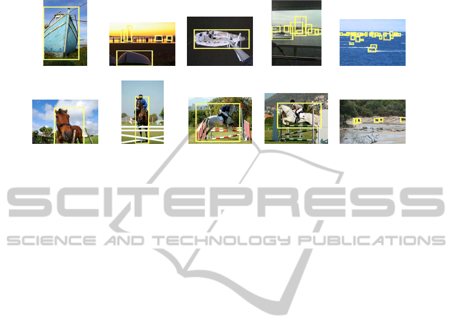
BOAT

HORSE

Figure 7: Heterogeneous shapes and sizes. This shows screen shots of VOC test images. The shots in the top row are for

the boat category and these in the bottom row are for the horse category. Yellow boxes are ground truth.

ACKNOWLEDGEMENTS

The research has been supported by the Natural Sci-

ences and Engineering Research Council of Canada

and the GEOIDE Network of Centres of Excellence,

Terrapoint Canada (A division of Ambercore).

REFERENCES

Abramson, Y. and Freund, Y. (2005). Semi-automatic vi-

sual learning (Seville): A tutorial on active learning

for visual object recognition. In CVPR.

Collins, B., Deng, J., Li, K., and Fei-Fei, L. (2008). To-

wards scalable dataset construction: An active learn-

ing approach. In ECCV.

Dalal, N. and Triggs, B. (2005). Histograms of oriented

gradients for human detection. In CVPR.

Everingham, M., van Gool, L., Williams, C., Winn, J., and

Zisserman, A. (2007). The PASCAL Visual Object

Classes Challenge 2007 (VOC2007) Results. http://

www.pascal-network.org/challenges/VOC/voc2007/

workshop/index.html.

Felzenszwalb, P. F., Girshick, R. B., McAllester, D., and

Ramanan, D. (2009). Object detection with discrimi-

natively trained part based models. PAMI.

Kapoor, A., Grauman, K., Urtasuna, R., and Darrrell, T.

(2007). Active learning with Gaussian processes for

object categorization. In ICCV.

Lazebnik, S., Schmid, C., and Ponce, J. (2006). Beyond

bags of features: Spatial pyramid matching for recog-

nizing natural scene categories. In CVPR.

Lewis, D. D. and Gale, W. A. (1994). A sequential algo-

rithm for training text classiﬁers. In Proc. of the 17th

annual international ACM SIGIR conference on Re-

search and development in information retrieval.

Moosmann, F., Larlus, D., and Jurie, F. (2006). Learning

saliency maps for object categorization. In ECCV.

Mutch, J. and Lowe, D. G. (2006). Multiclass object recog-

nition with sparse, localized features. In CVPR.

Qi, G.-J., Hua, X.-S., Rui, Y., Tang, J., and Zhang, H.-J.

(2008). Two-dimensional active learning for image

classiﬁcation. In CVPR.

Sch

olkopf, B. and Smola, A. (2002). Learning with Ker-

nels: Support Vector Machines, Regularization, Op-

timization and Beyond. MIT Press, Cambridge, MA,

USA.

Settles, B. (2010). Active learning literature survey. Tech-

nical Report 1648, University of Wisconsin-Madison.

Siddiquie, B. and Gupta, A. (2010). Beyond active noun

tagging: Modeling contextual interactions for multi-

class active learning. In CVPR.

Tong, S. and Koller, D. (2001). Support vector machine

active learning with applications to text classiﬁcation.

ML, 2:45–66.

Vijayanarasimhan, S., Jain, P., and Grauman, K. (2010).

Far-sighted active learning on a budget for image and

video recognition. In CVPR.

Vijayanarasimhan, S. and Kapoor, A. (2010). Visual recog-

nition and detection under bounded computational re-

sources. In CVPR.

Viola, P. and Jones, M. J. (2004). Robust real-time face

detection. IJCV, 57(2):137–154.

Zhang, H., Berg, A. C., Maire, M., and Malik, J. (2006).

SVM-KNN: Discriminative nearest neighbor classiﬁ-

cation for visual category recognition. In CVPR.

Zhang, L., Tong, Y., and Ji, Q. (2008). Active image la-

beling and its application to facial action labeling. In

ECCV.

VISAPP 2011 - International Conference on Computer Vision Theory and Applications

258