GENERATION OF PROCESS VARIANTS

Christiane Soika, Tobias Teich, Joerg Militzer and Daniel Kretz

Academic Department of Economics, University of Applied Sciences Zwickau, Zwickau, Germany

Keywords:

CAD, CAM, STEP, Ant colony optimization.

Abstract:

Small and medium sized enterprises (SME’s) are commonly dependent on large-scale enterprises in their

role as a supplier. In fact, growing international competition increases the pressure on SME’s. Hence, it is

enormously important, to react as fast and exact as possible on customer demands, while keeping high quality

standards atthe same time. In order to achieve these objectives, CAPP (Computer Aided Production Planning)-

systems were introduced. This paper provides an integrated solution for automated process and production

planning and we present our approach for generating process variants by using Ant Colony Optimization

(ACO).

1 INTRODUCTION

Inefﬁcient production planning in small and medium

sized enterprises (SME’s) is commonly known but

still a signiﬁcant problem. Generally, an integrated or

automated production planning is entirely missing for

small-series or single-part production. In their role

as a supplier it is existential, not only to react fast

and ﬂexible on customer demands, but also to provide

high quality products. Furthermore, it is very impor-

tant to reduce or completely avoid additional costs by

preventing the manufacturing of deﬁcient products.

These issues require an intelligent and very efﬁ-

cient organized production planning. CAPP-systems

are a fundamental component for an optimized pro-

duction planning within SME’s. This paper presents

our approach for integrating computer aided produc-

tion planning (CAPP) systems directly with computer

aided design (CAD) and enterprise resource plan-

ning (ERP) systems forevaluatingproduction variants

within a given factory environment.

1.1 Process Model for Integrated and

Automated Production Planning

Our intended solution for the introductory outlined

problem consists of ﬁve modules that are visualized

in terms of an extended event-driven process chain

(eEPC) in Figure 1 and Figure 2. First of all, there

is the Design Module (DM) that is used for providing

a CAD model of either a single piece part or complex

assemblies. Regarding this, we utilize the ISO stan-

dard 10303, most informally known as STEP ‘Stan-

dard for the Exchange of Product model data’. Be-

sides a standardized exchange, application protocols

of ISO 10303 provide reference models for a stan-

dardized product data representation. Thereby, we

have focused our attention on the reference model of

the application protocol 224 that is a special part of

ISO 10303 for machining industries (South Carolina

Research Authority, 2006). Within AP 224 ‘Mechan-

ical product deﬁnition for process planning using ma-

chining feature’ parts are modeled and parameterized

by using feature based design with machining fea-

tures.

Machining features are objects, whose semantics

imply corresponding manufacturing operations, like

a pocket feature implies a milling operation or an

outer diameter feature could indicate a turning oper-

ation. After deﬁning a base shape which deﬁnes an

initial volume, the ﬁnal part geometry is derived by

applying manufacturing features which describe vol-

umes that shall be removed by machining or shapes

that result from machining. Manufacturingfeatures of

ISO 10303 are classiﬁed into machining, replicate and

transition features. Furthermore, machining features

are specialized as compound or multi-axis features.

Compound features consist of two or more manufac-

turing features and multi-axis features are commonly

manufactured by milling processes. Transition fea-

tures deﬁne a transition area between at least two sur-

Soika C., Teich T., Militzer J. and Kretz D..

GENERATION OF PROCESS VARIANTS.

DOI: 10.5220/0003516100730078

In Proceedings of the 8th International Conference on Informatics in Control, Automation and Robotics (ICINCO-2011), pages 73-78

ISBN: 978-989-8425-74-4

 2011 SCITEPRESS (Science and Technology Publications, Lda.)

faces and replicate features are identical copies of any

arbitrary manufacturing feature or another replicate

feature.

Second, there is the Resource Description Module

(RDM) that is used for interpreting the design model

and determining alternative sets of required resources

and manufacturing operations for any involved man-

ufacturing feature (Gaese and Winkler, 2009), (Te-

ich et al., 2009). This module is additionally fed by

an ERP system, in our case the SAP system. The

RDM associates suitable manufacturing processes to

the corresponding manufacturing features from the

given product design model.

Figure 1: Automated process planning system (eEPC 1/2).

This n:n relation provides the input information

for our Graph Constructor Module (GCM) that gen-

erates process variants. Each process variant is sched-

uled and evaluated by a genetic algorithm (GA) of

our Evolutionary Module (EM). After a ﬁrst evalua-

tion, the GCM constructs alternative process variants

driven by the evaluated scheduling result and an ant

colony algorithm within our Swarm Intelligence Mod-

ule (SIM). The generation and evaluation of process

variants is an iterative process.

It is the matter of fact, that every manufacturing

feature that is used for destructive designing the part,

exponentially increases the number of process vari-

ants because we do not only derive variants from man-

ufacturing features themselves but also consider the

resulting part as a whole. Consequently, we utilize ar-

tiﬁcial intelligence, especially Ant Colony Optimiza-

tion (ACO) and GA, for the generation and evaluation

of these variants. The ACO selects a set of process

variants in cooperation with the GCM. Afterwards,

each set is scheduled considering manufacturing ca-

pacity during a potential production time, claimed de-

livery date and further target criteria. This process

requires information that is received from the SAP

system via Core Interface Function (CIF) through the

SAP Java Connector (SAP JCo).

Figure 2: Automated process planning system (eEPC 2/2).

Accruing costs, the entire production time and ad-

herence to delivery dates are primarily focused during

our evaluation. Afterwards, these variants are com-

pared with each other. This results into a steered

selection and generation of new process variants for

further evaluation. Consequently, these process steps

are repeated iteratively until any determination crite-

rion or certain target criteria are met. After deriving a

process variant that ﬁts the target criteria of costumer

and management, this solution is preserved. Further

details about the generation of process variants with

ACO are presented in detail within section 3.

1.2 Sequencing in Production Planning

The objective of sequencing is the determination of

a required manufacturing process sequence by us-

ing applicable machines (Loedding, 2005). Conse-

quently, sequencing always inﬂuences logistic target

values like delivery reliability, service level and yield.

Finally, there are two approaches for creating an ad-

vantageous sequence. There are mathematic deﬁnite

methods like branch and bound or the utilization of

heuristics like ant colony optimization or genetic al-

gorithms. The following sections discuss a concep-

tual solution for creating optimized sequences with

ICINCO 2011 - 8th International Conference on Informatics in Control, Automation and Robotics

heuristic methods.

2 PROCESS VARIANTS

In this issue, we want to focus our attention on creat-

ing sequences of manufacturing processes for produc-

ing single piece parts by turning, drilling or milling

operations. Subsequently, scheduling will be involved

for an evaluation of the generated process variants.

There are different target criteria to consider during

evaluation, like accruing production costs or adher-

ence to delivery dates for avoiding contractual penal-

ties. For our intended solution - to generate process

plans directly from a CAD drawing - we utilize the

feature-based design with manufacturing features be-

cause otherwise an efﬁcient and automated interpre-

tation of a complete and enhanced product design

model is absolutely hampered (Kretz et al., 2009).

Figure 3 illustrates required manufacturing fea-

tures of a roll-axis demonstrator. In fact, there are 21

features deﬁned for the ﬁnal shape. Considering, that

there may be several machines which could manufac-

ture the shape of one or many features with distinct

parameters for set-up time, accruing costs or process-

ing time, are facts increasing determination complex-

ity. To give an example for alternative machines, fea-

ture FE7 is an outer round-outer diameter that could

be manufactured either by a CNC-machining center

or a lathe. Furthermore, there could be technological

dependencies between feature aspects which shall be

minded.

Figure 3: Roll-axis with manufacturing features.

2.1 Feature Dependencies

Dependencies are distinguished between technologi-

cal and geometrical dependencies. The inﬂuence of

geometrical dependencies for process variant gener-

ation is low. But they are very important for the re-

sulting quality of a part. An example for geometrical

dependencies are FE20 and FE21. Both shall be man-

ufactured on exactly the same position on the left as

well as the right side of the part and right angular to

FE18. Inexactnesses and irregularities lead to a deﬁ-

cient part, which ﬁnally cannot be used.

Instead of this, a technological dependency is

given, if at least one feature requires the manufac-

turing of shape aspects deﬁned by other features.

Against geometrical dependencies, technological de-

pendencies inﬂuence process variants intensively. An

example for technological dependencies are the fea-

tures FE21 and FE16. FE21 is a round hole with

conical hole bottom and has to be manufactured ﬁrst.

FE16 typiﬁes a thread feature and could be only ap-

plied after drilling the hole. Consequently, we have

priorities that shall be considered for generating tech-

nological useful process variants.

Further restrictions are required for sequences

which could be technological manufactured but the

generated variant would be obviously inefﬁcient. To

give an example, a chamfer feature (FE12) could

maybe manufacturedbefore an associated outer diam-

eter (FE11) feature, but this is extremely inefﬁcient.

2.2 Graph Theory

For generating process variants we require a graph

representation. Features that shall be applied to man-

ufacture the ﬁnal part are deﬁned by the product

model. Consequently, our sequence graph is given

implicitly. Edges determine the application of man-

ufacturing features. Weighting of an edge depends

on the target criteria. Criteria are e.g. production

costs, time or a weighted combination of them. Fur-

thermore it has to be considered if a manufacturing

feature could be applied with a single manufacturing

operation.

Knots within our graph represent intermediate

products during the manufacturing of the part. Given

this fact, we have a dynamic graph. Depending on

the previous selection of features, the succeeding in-

termediate products are different. Therefore, we con-

struct our graph dynamically while generating a pro-

cess variant. The initial knot of our graph is always

deﬁned by the base shape. Considering feature de-

pendencies, there are still many variant edges remain-

ing. Each intermediate product depends on the se-

lected feature.

Feature selection and determination of the result-

ing intermediate product are repeated iteratively un-

til the part is completely manufactured. Possibly the

application of one manufacturing feature requires at

least more than one manufacturing operation. Hence,

a manufacturing operation only prepare part aspects

and succeeding operations complete the shape. Gen-

erating process variants in this way is very similar to

the Traveling Salesman Problem (TSP). Considering

GENERATION OF PROCESS VARIANTS

TSP, knots are cities that have to be visited and edges

dimension the distance between two cities. The objec-

tive is to ﬁnd the shortest round trip by visiting each

city exactly once. Both problems are very similar but

instead of our dynamic graph representation, the TSP

graph is static. Thus, the entire graph is traversable

every time and paths are ﬁxed. Best performance and

efﬁciency for solving such represented minimization

problems are achieved by ant colony optimization. In

1991, the Italian mathematician Marco Dorigo pub-

lished the ﬁrst ant algorithm for solving this problem

(Dorigo et al., 1991) (Dorigo and Stuetzle, 2004).

3 ANT COLONY OPTIMIZATION

Because the analogy of both problems, traveling

salesman and generation of process variants, we uti-

lize ant colony optimization. ACO is suitable for solv-

ing difﬁcult discrete optimization problems that could

be described by a graph. Therefore, we use simple

agents, in this case artiﬁcial ants who communicate

with each other mediated by the environment.

Our previously discussed problems are classiﬁed

as static and dynamic combinatorial problems. TSP

is a static combinatorial problem, because the initially

given information cannot change. Against this, the

generation of process variants is a dynamic combi-

natorial problem. An example for changing informa-

tion are the intermediate products. Depending on the

preceding selected features, the resulting intermediate

product is quite different. In fact, shape aspects of one

feature could not be manufactured with a single oper-

ation because a particular machine is unavailable or

against this, a compound-feature that consists of two

or more atomic manufacturing features could be man-

ufactured with a single operation on a special milling

center. This forces our algorithm, to adapt the chang-

ing problem deﬁnition (Dorigo and Stuetzle, 2004).

Ant colony optimization was already used for solving

similar kinds of problems, like optimizing production

plans (Liu et al., 2010) or ad-hoc-networks (Kamali

and Opatrny, 2009). ACO summarizes a set of dis-

tinct algorithms that are based on the same approach

but optimized for special problems. For our purposes,

we apply the Ant Colony System (ACS).

3.1 Ant Colony System

Ant Colony Optimization is a nature analogue ap-

proach that imitates the behavior of Argentine ants.

Ants have limited opportunities to communicate with

each other. They use a chemical substance for com-

munication called pheromones and deposit these on

their way between anthill and source of food. Con-

sequently, succeeding ants can orient themselves on

the given trace. If there are two different ways with

different lengths between anthill and source of food

source, the ﬁrst ant takes a random selection. A lit-

tle later, the pheromone concentration on the shorter

trace is higher than on the longer because of the length

this route could be more often passed. Consequently,

the probability of selecting the shorter route increases

with the pheromone concentration. But there always

remains a probability for selecting alternative routes

that characterizes a heuristic method. In fact, there is

never guaranteed that those algorithms ﬁnd the opti-

mal solution but they always have an optimizing na-

ture. Hence, the natural approach was scientiﬁcally

adapted for solving combinatorial problems. Ant al-

gorithms consist of three phases, starting with solu-

tion construction, followed by pheromone update and

optional daemon-activities.

For creating a solution, an ant starts from the cur-

rent initial knot with a speciﬁc probability to a neigh-

bored knot. Afterwards, this task is repeated until

a termination criterion is met. During pheromone

update, the ant deposits pheromone by leaving the

edge. Daemon-activities are further optional activi-

ties e.g. deposition of pheromones on the entire ﬁ-

nal ant path. Certain aspects of Ant Colony System

(ACS) differ from ant algorithm. To give an exam-

ple, ACS uses a global and a local pheromone update.

A global pheromone update addresses the deposition

and evaporation on the entire path of the current best

solution. Consequently, only the best evaluated ant is

authorized for a global pheromone update. Further-

more, there is a local pheromone update where every

ant reduces the pheromone concentration after leav-

ing an edge. This approach supports a wide search

that avoids a concentration on local optima as well as

premature convergence (Fischer, 2008).

Figure 4: Pseudo code for generating process variants.

ICINCO 2011 - 8th International Conference on Informatics in Control, Automation and Robotics

3.2 Algorithm for Generating Process

Variants

Listing 4 presents the pseudo code of our process vari-

ant generation approach. First of all, a suitable raw

material and the base position of the ﬁnal part are de-

termined. Against the default ant algorithm, our ap-

proach upgrades the ants with a memory about the

manufacturing features of the part and their techno-

logical dependencies (feature list). After determin-

ing the raw material, each ant decides which feature

shall be manufactured ﬁrst. Therefore, it has to be

checked whether there is already pheromone on this

edge. Hence, we check for every feature in the list,

whether there is a pheromone value on the edge be-

tween initial shape and resulting intermediate prod-

uct. If there is no pheromone value for orientation,

the selection is straight randomly. Otherwise the se-

lection is weighted as a pheromone-steered random

selection.

The probability p(x

), for selecting an edge from

either an initial base shape or an intermediate product

i to a further intermediate product j is derived by the

following formula:

p(x

) =

· ν

∑

k∈X

· ν

(1)

represents the pheromone concentration on the

edge between intermediate product i and j. The

parameters α and β inﬂuence the concentration of

pheromone and heuristic information (Kramer, 2009).

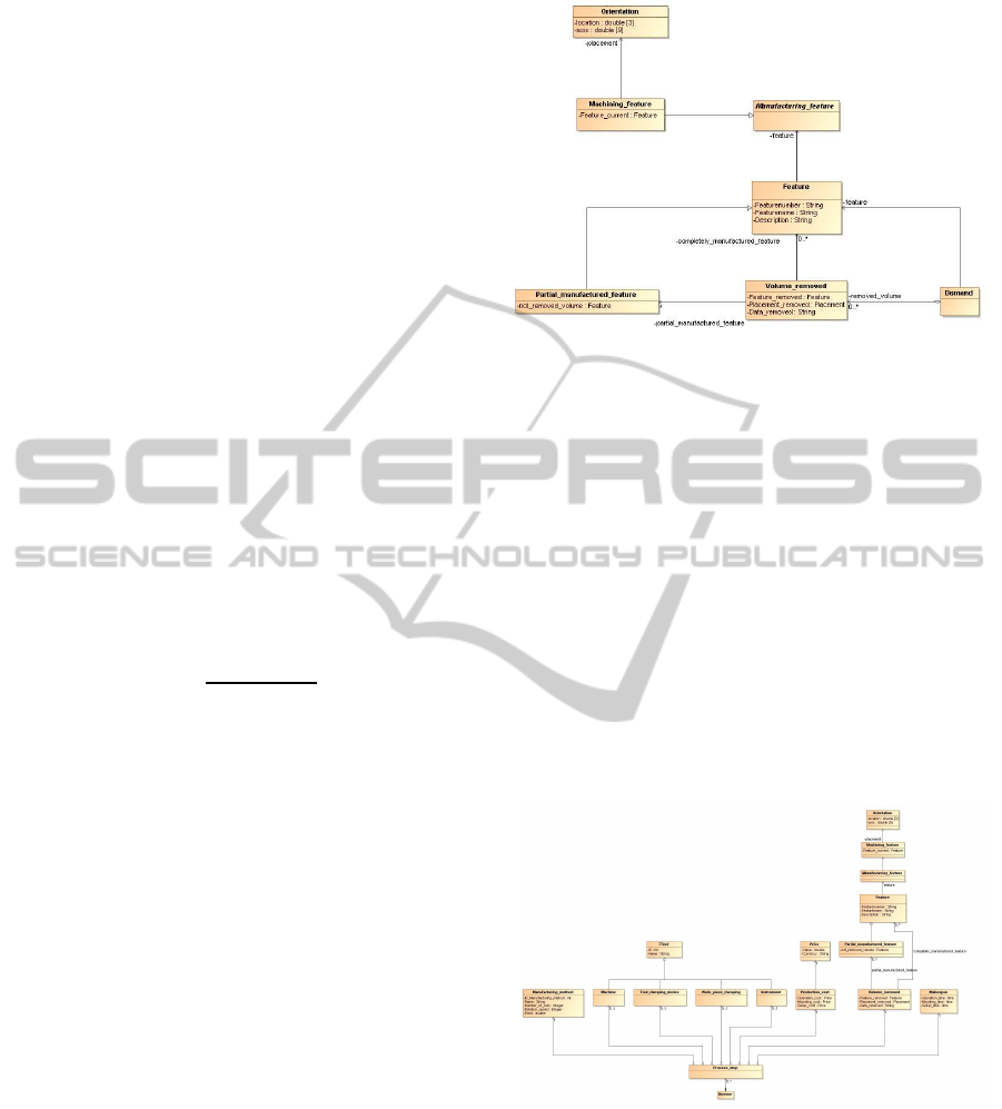
After selecting an edge for the next step, it has to

be checked whether technological dependencies pre-

vent the manufacturing of the involved feature or not.

If there are not any technological dependencies, the

location and orientation of a feature are derived and

requested as a demand to our RDM. The correspond-

ing data structure is illustrated as class diagram in Fig-

ure 5.

The demand consists of two parts. First, there is

the feature information like identiﬁer, name, descrip-

tion, location, orientation and other required parame-

ters. Those are used by the RDM for determining a set

of suitable manufacturing operations. Second, their is

an information about the concrete previous selection

from this set. Hence our RDM updates the current

intermediate product.

After determining suitable manufacturing opera-

tions, the set is replied as an answer as illustrated in

Figure 6. Possibly, there are no suitable manufac-

turing operations, e.g. if there currently is not any

machine available or a single manufacturing opera-

tion could apply more than one features. If an answer

Figure 5: UML class diagram: feature request.

contains at least one operation, then it supplies the

following information:

• removed volume,

• state of manufacturing,

• manufacturing method,

• selected machine,

• used tool,

• required tool clamping devices,

• required work piece clamping,

• production time (execution, mounting and set-up)

• production costs (execution, mounting and set-

up).

Figure 6: UML class diagram: RDM answer.

Driven by the target criteria, one of the opera-

tions are selected. The selection depends on time-

or cost-minimization or a composition of them. An-

other aspect is the state of manufacturing that indi-

cates whether a feature was manufactured completely

or not. If it was only prepared, hence a further pro-

cess step is later required for completion. Otherwise,

it was manufactured completely and consequently re-

moved from feature list. Afterwards, evaporation is

GENERATION OF PROCESS VARIANTS

utilized, if there is pheromone on the edge. Without

evaporation, the search would result in a premature

convergence on a local optimum. The evaporation is

calculated with the following formula:

= (1 − ϕ) · τ

(2)

ϕ is a parameter which describes the evaporation

rate, deﬁned by 0 < ϕ < 1 (Fischer, 2008).

Selection of the next feature, request to and re-

sponse from RDM, as well as the selection of a manu-

facturing operation from the response set are repeated

until the entire process variant is generated and thus

the ﬁnal part produced. Afterwards, the process vari-

ant is preserved and evaluated with our GA. If the

current process variant is the best, then pheromones

are deposited on the entire path. Currently, we have

only focused production time and accruing costs of

the manufacturing operations. In fact, there are still

another aspects. To given an example, two features

have to be manufactured on two different machines.

The resulting intermediate product has to be trans-

ported from current machine to another. Hence, this

additional time and consequently it could be more ef-

ﬁcient to execute both operations on the same ma-

chine.

4 CONCLUSIONS

We have stated our problem of generating process

variants in an automated integrated production plan-

ning within this paper. Therefore, we have geomet-

rical and technological dependencies deﬁned which

derive from the feature based design. For solving our

generation problem, we utilize heuristic approaches,

especially ant colony optimization and genetic algo-

rithms. This paper provided a short introduction about

Ant Colony Optimization and our intention for their

usage. Finally, we have explained our approach for

generating process variants with the Ant Colony Sys-

tem. Future work deals with the implementation and

integration of this approach into our planing solution

as a software module.

REFERENCES

Dorigo, M., Maniezzo, V., and Colorni, A. (1991). Ant

system: An autocatalytic optimizing process.

Dorigo, M. and Stuetzle, T. (2004). Ant Colony Optimiza-

tion. MIT Press.

Fischer, M. (2008). Partnerauswahl in netzwerken. Verlag

Dr. Kovaˇc.

Gaese, T. and Winkler, S. (2009). Entwicklung eines

ressourcenmodells fr die automatische angebots-

generierung auf grundlage featurebasierter produk-

tbeschreibung. In Journal of the University of Applied

Sciences Mittweida, pages pp. 18–21. Hochschule

Mittweida.

Kamali, S. and Opatrny, J. (2009). A hybrid ant-colony

routing algorithm for mobile ad-hoc networks. In

Complex Sciences, pages pp. 1337–1354. Springer,

Berlin Heidelberg.

Kramer, O. (2009). Computational Intelligence. Springer

Verlag.

Kretz, D., Teich, T., Militzer, J., Jahn, F., and Neumann, T.

(2009). Step standardized product data representation

and exchange for optimized product development and

automated process planning. In Proceedings of the 6th

CIRP-Sponsored International Conference on Digital

Enterprise Technology, pages pp. 41–56. Springer.

Liu, X., Yi, H., and Ni, Z. (2010). Application of ant colony

optimization algorithm in process planning optimiza-

tion. In Journal of Intelligent Manufactoring, pages

pp. 1–13.

Loedding, H. (2005). Verfahren der fertigungssteuerung.

Springer Verlag.

South Carolina Research Authority (2006). STEP

Application Handbook ISO 10303. SCRA/ISG,

5300 INTERNATIONAL BOULEVARD. NORTH

CHARLESTON, SC 29418, 3. version edition.

Teich, C., Duerr, H., Militzer, J., Neumann, T., and Tran, N.

(2009). Automatische grobkalkulation auf basis funk-

tionaler beschreibung der nachfrage. In Logistics and

Supply Chain Management - Modern Trends in Ger-

many and Russia, pages pp. 294–305. Cuvillier Verlag

Goettingen.

ICINCO 2011 - 8th International Conference on Informatics in Control, Automation and Robotics