A PARALLEL HEURISTIC FOR FAST TRAIN DISPATCHING
DURING RAILWAY TRAFFIC DISTURBANCES: EARLY RESULTS
Syed Muhammad Zeeshan Iqbal, H˚akan Grahn and Johanna T¨ornquist Krasemann
School of Computing, Blekinge Institute of Technology, SE-371 79 Karlskrona, Sweden
Keywords:
Railway traffic, Disturbance management, Optimization, Re-scheduling, Parallel computing, Multiprocessor.
Abstract:
Railways are an important part of the infrastructure in most countries. As the railway networks become more
and more saturated, even small traffic disturbances can propagate and have severe consequences. Therefore, ef-
ficient re-scheduling support for the traffic managers is needed. In this paper, the train real-time re-scheduling
problem is studied in order to minimize the total delay, subject to a set of safety and operational constraints.
We propose a parallel greedy algorithm based on a depth-first branch-and-bound search strategy. A number of
comprehensive numerical experiments are conducted to compare the parallel implementation to the sequential
implementation of the same algorithm in terms of the quality of the solution and the number of nodes eval-
uated. The comparison is based on 20 disturbance scenarios from three different types of disturbances. Our
results show that the parallel algorithm; (i) efficiently covers a larger portion of the search space by exchang-
ing information about improvements, and (ii) finds better solutions for more complicated disturbances such as
infrastructure problems. Our results show that the parallel implementation significantly improves the solution
for 5 out of 20 disturbance scenarios, as compared to the sequential algorithm.
1 INTRODUCTION
Railways are an important part of the infrastructure
in most countries. As the railway traffic networks
become more and more saturated, even small traf-
fic disturbances can propagate and have severe con-
sequences. Smooth operation of railway systems
are also difficult due to different types of unforeseen
larger disturbances such as bad weather or infrastruc-
ture failures. When disturbances occur, the timetable
needs quickly to be re-defined to minimize the de-
lays and the associated penalty costs for operators and
infrastructure providers. However, the large number
of constraints and complex infrastructure make re-
scheduling difficult and time consuming. Therefore,
efficient re-scheduling support for the traffic man-
agers is needed.
In Sweden, the railway transport market is dereg-
ulated which means that operators and infrastructure
providers are two different entities. The Swedish
Transport Administration, Trafikverket, is managing
the network both in terms of timetabling and traffic
management while the operators arrange and run the
train services for passengers and freight. The different
private operators apply for desirable slots in competi-
tion with each other and Trafikverket assigns slots ac-
cording to predefined market-based routines. The de-
mand for track capacity has increased the past years in
Sweden as well as the number of operators (T¨ornquist
and Persson, 2007). As an effect, the network is be-
coming more and more saturated and vulnerable every
year. The Swedish railway industry therefore seeks
decision support systems to assist dispatchers in mak-
ing good re-scheduling and delay management deci-
sions in real time. Since this re-scheduling problem is
a difficult problem, solution approaches based on e.g.
traditional optimization techniques often require huge
amount of memory space and computation time. Es-
pecially the computation time is important to reduce
since the problem needs to be solved fast in real-time.
The purpose of this paper is to present a fast and
effective approach for railway traffic re-scheduling
which aims to minimize the delays during a distur-
bance by the use of heuristics and parallelization tech-
niques. The approach is a parallel depth-first search
(DFS) branch-and-bound (B&B) algorithm based on
a sequential greedy algorithm proposed by (T¨ornquist
Krasemann, 2010; Grahn and T¨ornquist Krasemann,
2011). The parallel DFS algorithm has been evaluated
experimentally and benchmarked with the sequential
greedy version as well as to state-of the art optimiza-
tion software, Cplex 12.2, for 20 disturbance scenar-
405
Muhammad Zeeshan Iqbal S., Grahn H. and Törnquist Krasemann J..
A PARALLEL HEURISTIC FOR FAST TRAIN DISPATCHING DURING RAILWAY TRAFFIC DISTURBANCES: EARLY RESULTS.
DOI: 10.5220/0003756904050414
In Proceedings of the 1st International Conference on Operations Research and Enterprise Systems (ICORES-2012), pages 405-414
ISBN: 978-989-8425-97-3
Copyright
c
 2012 SCITEPRESS (Science and Technology Publications, Lda.)

ios. The simulated disturbance scenarios are used to
measure the algorithm efficiency in terms of the qual-
ity of the solution and the number of nodes explored.
Our results show that the parallel implementation sig-
nificantly improves the solution for 5 out of 20 distur-
bance scenarios, as compared to the sequential algo-
rithm.
In the following section, related work is presented.
Section 3 outlines the problem domain and its context
as well as a description of the sequential greedy algo-
rithm. Sections 4 and 5 present the parallel algorithm
and the experiments performed to analyze its perfor-
mance, respectively. In Section 6, the experimental
results are presented and discussed. Finally, Section 7
concludes our study and provides suggestions for fu-
ture work.
2 RELATED WORK
The railway traffic delay management and re-
scheduling problem has been considered an important
and difficult problem since quite some time. Com-
prehensive reviews of related work can be found in,
e.g., (T¨ornquist, 2005; Conte, 2008; Schachtebeck,
2009) and it has been studied from different perspec-
tives such as capacity, robustness, as well as passen-
ger delay and dissatisfaction. Analysis of heuristics
and integer solution methods for solving capacitated
re-scheduling delay management problems are given
in, e.g., (Schachtebeck, 2009).
The capacitated delay management prob-
lem (Schachtebeck, 2009) is a special case of the
job shop scheduling (JSS) problem, where train
trips are jobs which are scheduled on tracks that
are considered as resources. A JSS formulation is
also proposed in (Liu and Kozan, 2009) where a
blocking parallel-machine JSS is used to model the
train dispatching.
A branch and bound (B&B) procedure is proposed
for a resource-constrained project scheduling formu-
lation by incorporating an exact lower bound rule and
a beam search heuristic for a tight upper bound (Zhou
and Zhong, 2007). A four step heuristic is proposed
in (Lee and Chen, 2009), in which binary integer lin-
ear programming is used to accept or reject proposed
solutions.
More recently, the delay management problem has
been studied by (Corman, 2010), where the com-
plexity of dispatching is discussed, and mathemati-
cal models, based on an alternativegraph formulation,
along with algorithm enhancements are proposed. A
similar problem, but with a different problem setting,
is studied in (T¨ornquist and Persson, 2007) where
an Mixed-Integer Linear Program (MILP) formula-
tion for dispatching trains during disturbances is pro-
posed and solved using commercial software. The
MILP model showed to be too time-consuming to
solve using existing commercial solvers for more se-
vere disturbances. Therefore, a greedy depth-first
search branch-and-bound algorithm was developed
for addressing the re-scheduling problem (T¨ornquist
Krasemann, 2010) and further improved in (Grahn
and T¨ornquistKrasemann, 2011) with a more efficient
branching strategy.
In (Grama and Kumar, 2002), a survey of parallel
search methods in combinatorial optimization prob-
lems (COP) in connection to artificial intelligence is
presented. The work in (Clausen and Perregaard,
1999) can be considered as an extension of (Grama
and Kumar, 2002), while adopting the same search-
ing methods (i.e. DFS or BFS) with B&B. Branch-
ing strategies named lazy and eager (i.e. in eager,
branching is performed before bound calculation but
in lazy vice versa) are introduced with performance
results (Clausen and Perregaard, 1999). The search
procedures are improved by parallel implementations
on multiprocessors in the context of constraint pro-
gramming (Perron, 2004). The advantages and disad-
vantages of central or distributed together with mixed
control schemes for implementation of parallel B&B
are discussed (Shinano et al., 1997). Further, a par-
allel search engine has been devised using different
time limits (Perron, 2004).
The focus of this paper is different from related re-
search in other countries since the complete Swedish
railway network permits bi-directional traffic. Fur-
thermore, on double-tracked line sections track swap-
ping and using both tracks for traffic in one direc-
tion is a commonly used traffic management strategy
when re-scheduling the traffic during disturbances.
These properties complicate the problem and make it
harder to solve. Furthermore, the application of paral-
lelization has not been previously addressed to solve
the real-time railway re-scheduling problem.
3 PROBLEM DESCRIPTION AND
SEQUENTIAL GREEDY
ALGORITHM
3.1 Railway Network Representation
The railway network consists of station and line sec-
tions, tracks, blocks, and events. Each station and
line section can have one or more parallel tracks. All
tracks are bi-directional, i.e., the track can be used
ICORES 2012 - 1st International Conference on Operations Research and Enterprise Systems
406

for traffic in both directions depending on the sched-
ule. A train uses exactly one track on a station or
line section, but which specific track to use is often
only predefined for events on stations where the cor-
responding train has a passenger stop. The track allo-
cation is therefore a part of the re-schedulingproblem.
Each track is composed of one or several blocks con-
nected serially and separated by signals. Each block
can hold only at most one train at a time due to the
safety restriction imposed by line blocking. A track
composed of two blocks can in theory hold two trains
in the same direction, but not two trains in opposite di-
rection due to the lack of a meeting point. Each train
has an individual, fixed route (i.e. the sequence of sec-
tions to occupy) which is represented as a sequence of
train events to execute. A train event is when a certain
train occupies a certain section. A train event has cer-
tain static properties such as minimum running time,
advertised start and end times (i.e. it can not depart
earlier than the advertised departure time) and rec-
ommended track at stations with passenger connec-
tions. The event has also some dynamic properties,
e.g., track allocation and start and end times on the
section.
3.2 Problem Specification
In the train re-scheduling problem we have a dis-
turbance in the railway traffic network forcing us
to modify the predefined timetable in line with cer-
tain objective(s) and constraints. We have a set of n
trains, T = {t
1
, t
2
, . . . , t
n
} on a set of m sections, S =
{s
1
, s
2
, . . . , s
m
} where each section s
j
∈ {station, line}
have a number of tracks p ∈ {1, . . . , p
j
}. A station is
called symmetric if the choice of track to occupy has
no, or negligible, effect on the result. Each train i has
a set of events, K
i
and the set of all train events is
denoted as K = {K
1
, K
2
, . . . , K
n
} and its cardinality is:
C =
∑
|T|
i=1
|K
i
|. Each train event k has a predefined start
time t
start
k
and end time t
end
k
in line with the timetable
and which needs to be modified based on the mini-
mum running time d
k
. It also belongs to a specific
section s
k
∈ {s
1
, s
2
, . . . , s
m
}. Each event is executed
on exactly one track of its section.
In Figure 1, 9 trains are shown. Train A has 7
events and each event is associated with a section
(e.g., A1 at section 1). There are totally 7 sections,
where sections 1, 3, 5, and 7 are stations and sections
2, 4, and 6 are line sections.
The objective of the re-scheduling procedure is to
minimize the sum of the final delay suffered by each
train at its final destination within the problem in-
stance. The quality of the solution is thus given by
this objective value, where a lower value indicates an
Figure 1: Illustration of railway traffic on a double-tracked
line with four stations and three line sections. The time
stamp T
0
indicates the time when Train C just has left sec-
tion 1 and experiences an engine failure. The itinerary of
Train C will then look different than from the planned one.
improvement. The optimal solution is the one found
by the optimization software (Cplex 12.2 in our case).
The search space explored is quantified by the number
of nodes visited.
3.3 A Sequential Greedy Algorithm
The main objective of the sequential greedy algorithm
is to quickly find a feasible solution, and therefore
it performs a depth-first search. It uses an evalua-
tion function to prioritize when conflicts arise and
branches according to a set of criteria. When a first
feasible solution has been found the algorithm contin-
ues to search for improvements if the time limit per-
mits it. In our experiments we have set the time limit
to 30 seconds. A detailed description of algorithm
with pseudo code and examples is given in (T¨ornquist
Krasemann, 2010).
A search tree is built iteratively by selecting the
earliest event of each train, collecting them into a
sorted candidate list, assessing which event to exe-
cute first and executing the selected event. An event
represents a train movement, i.e., a train running on a
certain section with a start time, a minimum running
time, a preferred track to occupy, and an end time.
Each node in the search tree represents an active or
terminated event ( i.e.the train has left the assigned
track and either started the next event or reached its
final destination). For each node, we compute an op-
timistic estimation of the minimum cost, CV, for the
final solution given the partial solution that the branch
corresponds to. The further down in the tree a node
is located, the more exact the estimation becomes and
consequently nodes at maximum depth holds a cost
A PARALLEL HEURISTIC FOR FAST TRAIN DISPATCHING DURING RAILWAY TRAFFIC DISTURBANCES:
EARLY RESULTS
407

estimation value which corresponds to the objective
value of that solution.
The tree building process is divided into three
phases: (i) pre-processing, (ii) depth-first search, and
(iii) solution improvement using backtracking and
branching on potential nodes. In the pre-processing
phase, all events which were active at the disturbance
time T
0
(see Figure 1) are executed by allocating a
start time and a track. A lower bound, LB, is defined
and assigned the value of CV for the end node in the
pre-processing phase tree. A sorted next candidate list
(i.e., sorted w.r.t the earliest possible starting time of
the event), denoted NC, holds the first waiting event
of each train. In the second phase, feasible (i.e., dead-
lock free, without conflicts, etc.) candidate events are
executed and removed from the candidate list one by
one. The next candidate list is updated accordingly
by adding the next waiting event of the train that just
executed an event (if it has any left to execute) and is
then re-sorted. The third phase starts as soon as the
first feasible solution has been found. It aims to im-
prove the best solution found so far by backtracking
to a potential node, where the estimated cost, CV, is
lower than the current best solution, and explores an-
other branch from there. The improvement process
continues until the time limit is reached or a feasible
solution with an objective value equal to LB is found.
4 PARALLEL DEPTH-FIRST
SEARCH BRANCH AND
BOUND ALGORITHM
Our parallel algorithm is based on the sequential
greedy algorithm described in Section 3.3, and where
the B&B procedure is improved by sharing improved
solutions among workers using a synchronized white
board. We use a master-slave parallelization strategy.
Initially, only the master is active and the workers
(slaves) are waiting to get the initial unexplored sub-
spaces. Using the notations in Table 1, we outline the
parallel algorithm starting with the master thread.
4.1 The Master Process
Let NC and PS be empty, and the disturbance occurs
at time T
0
. As in the sequential algorithm, identify
the events that are active at T
0
, execute them, and put
them into PS. Populate the NC with the next event to
execute of each train, sorted w.r.t the earliest starting
time, and compute the theoretical lower bound. De-
termine the values of T
c
and W where W = T
c
in these
experiments. A unique copy of the problem along
Table 1: Notation used in the parallel search.
Symbol Definition
NC = C
1
, C
2
, ..., C
n
where NC is the candidate
list
PS = partial solution branch
T
0
= the time when the disturbance occurs
ET
Limit
= execution time limit (30 sec in our exper-
iments)
C
i
= candidate index to start with
T
c
= total number of candidates
BV
w
= branching value
GBV = global best value communicated via the
white board
CV
w
= cost estimation value of the current node
W = total number of workers
w = worker index
S(w) = solution branch found by worker w
Figure 2: Parallelization at different depths in the search
tree.
with ET
Limit
, C
i
and PS are sent to each worker. Look-
ing at the example in Figure 1, PS contains A6, B4
and C2 (i.e., train A associated to section 6 as event
A6 etc.), while NC consists of A5, B5, C3, D1, E7,
F1, G1, H7, and I1. One candidate event each is as-
signed to the workers to start with. Figure 2 gives an
overview of how the parallelization is applied at dif-
ferent depths of the search tree.
4.2 The Worker Process
The outline of the worker process is as follows:
Candidate Selection. First execute the candidate C
i
,
determine the new NC and get a suitable candidate
based on the depth-first search node selection rule.
ICORES 2012 - 1st International Conference on Operations Research and Enterprise Systems
408

Stopping Criteria. If the bounds in terms of execu-
tion time limit ET
Limit
is exceeded or the lower bound
is reached, then terminate and output the best result. If
the candidate to execute, i.e., C
i
, is not suitable, then
stop execution and return.
Read White Board. Read the white board for avail-
ability of improved solutions found by any other
worker; if available, then update BV
w
in line with
GBV.
B&B Process. When the value of CV
w
is greater than
or equal to the value of GBV, discard the node, back-
track and try other alternatives, and discard branches
from symmetric stations (see Section 3.2).
Feasible Solution. If all of the train events are termi-
nated, then update the white board if the new solution
found is better than the previously best solution. With
an updated value of BV
w
, backtrack and start branch-
ing from a node with a value less than BV
w
.
Deadlock Handling. In case of no track availability,
backtrack to detect where the wrong decision possibly
was made, revoke this decision (i.e. the execution of
a certain event) and start branching from there.
Results. After termination, send back the solution
S(w) to the master.
5 EXPERIMENTAL SETUP
Our objective is to investigate a number of important
aspects through a series of numerical experiments:
(1) How does the parallelization point (i.e. at what
depth in the tree to start the parallel search) and, (2)
the number of workers affect the performance of the
parallel algorithm. Given the results from this anal-
ysis, indicating a suitable combination of paralleliza-
tion depth and number of workers, we also investigate
3) how the algorithm performs in comparison to solu-
tions found by the sequential algorithm and the com-
mercial solver Cplex 12.2. The performance analysis
is based on the metrics described in Section 3.2. In ad-
dition, we investigate how many improved solutions
that are found as compare to the sequential algorithm.
In our experimentswe consider a dense traffic area
of Sweden that consists of both single- and double-
tracked line sections as shown in Figure 3. All sec-
tions are bi-directional and several of them have mul-
tiple blocks. The 28 stations have 2 to 14 tracks
each except Norsholm with only one track. The sta-
tions
˚
Aby, Str˚angsj¨o, and Simonstorp are modelled in
more detail by defining all the forbidden paths into
and out of the stations explicitly, see Appendix B
in (T¨ornquist Krasemann, 2010)
For a systematic and comprehensive assessment
of the performance of the parallel algorithm, we have
Table 2: Description of the 20 disturbance scenarios.
No. Scenario description #trains/events/
binary variables
1 Long-distance pax train 538, north-bound, delay 12
minutes Link¨oping-Linghem.
50/549/8214
2 Long-distance pax train 538, north-bound, delay 6
minutes Link¨oping-Linghem.
50/549/8214
3 Pax train 2138, south-bound, delay 12 minutes
Katrineholm-Str˚angsj¨o.
50/553/8326
4 Pax train 2138, south-bound, delay 6 minutes
Katrineholm-Str˚angsj¨o.
50/553/8326
5 Pax train 80866 (north-bound), delayed 12 minutes
Link¨oping-Linghem.
51/565/8430
6 Pax train 80866 (north-bound), delayed 6 minutes
Link¨oping-Linghem.
51/565/8430
7 Pax train 8764 (north-bound), delayed 12 minutes
Mj¨olby-Mantorp.
52/556/8425
8 Pax train 8764 (north-bound), delayed 6 minutes
Mj¨olby-Mantorp.
52/556/8425
9 Pax train 539 (south-bound), delayed 12 minutes
Katrineholm-Str˚angsj¨o.
52/558/8369
10 Pax train 539 (south-bound), delayed 6 minutes
Katrineholm-Str˚angsj¨o.
52/558/8369
11 Pax train 538 w. permanent speed reduction causing
50% increased run times on line sections starting at
Link¨oping-Linghem
50/549/8214
12 Pax train 2138 w. permanent speed reduction caus-
ing 50% increased run times on line sections starting
at Katrineholm-Str˚angsj¨o.
50/553/8326
13 Pax train 80866 w. permanent speed reduction caus-
ing 50% increased run times on line sections starting
at Link¨oping-Linghem.
50/566/8382
14 Pax train 8764 w. permanent speed reduction caus-
ing 50% increased run times on line sections starting
at Mj¨olby-Mantorp.
52/556/8425
15 Pax train 539 w. permanent speed reduction causing
50% increased run times on line sections starting at
Katrineholm-Str˚angsj¨o.
52/558/8369
16 Speed reduction for all trains between Str˚angsj¨o and
Simonstorp (all trains get a runtime of 27 min, cf.
5-10 min planned runtime) starting w. freight train
43533.
48/509/7059
17 Speed reduction for all trains between
˚
Aby and Si-
monstorp (all trains get a runtime of 20 min) starting
w. train 2138.
53/558/8516
18 Speed reduction for all trains between
˚
Aby and
Norrk¨oping(all trains geta runtime of 8 min) starting
w. train 2138.
51/554/8224
19 Speed reduction for all trains between Mj¨olby and
Mantorp (all trains get a runtime of 20 min) starting
w. train 8764.
52/556/8224
20 Speed reduction for all trains betweenLink¨oping and
Linghem (all trains get a runtime of 15 min) starting
w. train 538.
50/549/8214
constructed 20 realistic disturbance scenarios. The
scenarios are presented in Table 2, and are slightly
modified from the scenarios in (T¨ornquist Krase-
mann, 2010). The few minor modifications made
are done to avoid that the event list of a train ends
with an event in the middle of a set of consecutive
line sections, e.g., as between the stations
˚
Aby and
Norrk¨oping. A small number of additional events are
therefore included in the scenarios used in this paper.
For a 90 minute long time horizon, the third column
in Table 2 shows the total number of trains be sched-
uled, the total number of events, and the number of
binary variables required for the corresponding MILP
formulation solved by Cplex. The disturbance scenar-
ios cover three types of disturbances:
1. Scenarios 1-10 have initially a temporary single
source of delay, e.g., a train comes into the traffic
management district with a certain delay, or it suf-
A PARALLEL HEURISTIC FOR FAST TRAIN DISPATCHING DURING RAILWAY TRAFFIC DISTURBANCES:
EARLY RESULTS
409

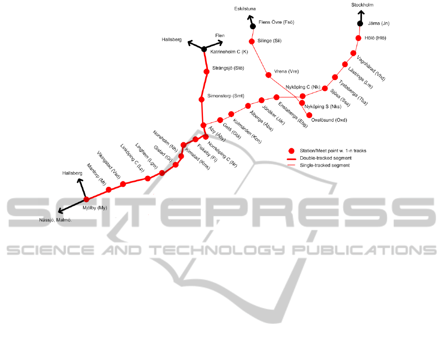
Figure 3: The traffic area in Sweden that are used in the study. It has in total 28 stations, all line sections are bi-directional,
wide lines indicate double-tracked sections, and thin lines single-tracked.
fers from a temporary delay at one section within
the district.
2. In scenarios 11-15, a train has a ’permanent’ mal-
function resulting in increased running times on
all line sections it is planned to occupy.
3. In scenarios 16-20, the disturbance is an infras-
tructure failure causing, e.g., a speed reduction on
a certain section, which results in increased run-
ning times for all trains running through that sec-
tion.
The sequential and parallel algorithms are im-
plemented in Java using the multithreaded API with
JDK 1.6, and all experiments are conducted on a
server running Ubuntu 10.04 and equipped with two
quad-core processors (Intel Xeon E5335, 2.0 GHz)
and 16 GB main memory. The execution time limit
ET
Limit
is set to 30 seconds. Cplex (version 12.2) was
run on a AMD Opteron(tm) 285 quad-core processor
and in parallel, deterministic mode with 4 threads and
given a time limit of 24 hours. We also set the time
limit for Cplex to 30 seconds, but it did not manage
to provide any feasible solution in all 20 disturbance
scenarios within this time.
6 EXPERIMENTAL RESULTS
In this section, the results from the experimental eval-
uation of the parallel algorithm are presented. First,
we analyze how the parallelization affects the per-
formance and at which parallelization depths solution
improvements are found. Secondly, a statistical anal-
ysis is made for the second performance metric, i.e.,
the number of visited nodes. This part of the evalu-
ation focuses on one very complex disturbance sce-
nario, i.e., scenario 20 in Table 2.
Finally, we compare the parallel algorithm with
the sequential algorithm and the optimal solutions
found by Cplex for all 20 disturbance scenarios.
Our evaluation metrics are the solution quality,
i.e., the sum of the final delay of all trains, and the
number of nodes explored, see Section 3.2 .
6.1 Analysis of Parallelization Depths
and Number of Workers
In the evaluation of how the number of workers and
the parallelization depth affect the solution quality,
we selected six different parallelization depths: at T
0
,
100, 200, 300, 400, and 500 nodes as shown in Fig-
ure 2. For each depth, we use 4 different sets of work-
ers containing 8, 16, 32, and the maximum number
of available candidates at the particular depth in the
search tree. Table 3, shows the experimental results
for all combinations of the number of workers and
the depth for disturbance scenario 20. In Table 3, the
different solutions are characterized by the worker id
(i.e. which worker found the solution), the associated
solution value, and the time to find that solution. The
minimum time to find an initial feasible solution and
maximum time to find an improved solution is 0.06
ICORES 2012 - 1st International Conference on Operations Research and Enterprise Systems
410

Table 3: Experimental results for scenario 20 using a time horizon of 90 minutes and 30 seconds execution time, for different
number of workers and parallelization depths.
Depth Nodes Solutions Nodes Solutions
visited (Worker id, cost, time) visited (Worker id, cost, time)
8 Workers 16 Workers
T
0
8 573 135 (2, 27208, 0.24), (3, 27186, 0.49), (0, 23609, 0.52),
(0, 23587, 0.83)
7 841 418 (5, 27208, 0.56), (11, 27186, 0.84), (1, 23609, 0.91),
(1, 23587, 1.22)
100 8 048 136 (7, 27186, 0.51), (0, 23609, 0.60), (5, 23587, 0.64) 8 381 525 (12, 27208, 0.14), (8, 27186, 0.56), (5, 23587, 0.77)
200 7 334 836 (3, 27186, 0.16), (2, 23587, 0.23) 8 440 333 (1, 27208, 0.18), (15, 27186, 0.24), (8, 23587, 0.41)
300 4 699 518 (6, 27208, 0.06), (5, 27186, 0.14), (7, 23587, 0.19) 7 816 092 (12, 27208, 0.07), (11, 27186, 0.34), (9, 23587, 0.47)
400 4 730 399 (5, 27186, 0.10), (4, 23587, 0.15) 7 790 739 (11, 27208, 0.07), (8, 27186, 0.21), (5, 23587, 0.30)
500 1 916 351 (6, 27186, 0.07), (7, 23587, 0.12) 1 986 419 (7, 27186, 0.09), (6, 23587, 0.16)
32 Workers Maximum number of Workers
T
0
6 817 627 (5, 27208, 1.27), (26, 26765, 1.10), (29, 23609, 1.65),
(26, 23166, 2.06), (26, 23144, 2.52)
5 722 240 (19, 27208, 1.03), (32, 26765, 1.14), (31, 23609, 2.34),
(26, 23166, 2.56), (26, 23144, 3.70)
100 7 065 428 (2, 27208, 0.34), (14, 27186, 1.45), (7, 23609, 1.59),
(1, 23587, 1.69)
6 668 677 (9, 27208, 0.33), (6, 27186, 1.43), (5, 23587, 1.83)
200 7 418 218 (1, 27208, 0.25), (28, 27186, 0.57), (3, 23587, 0.83) 7 160 066 (4, 27208, 0.17), (7, 27186, 0.70), (18, 23587, 0.72)
300 6 626 197 (6, 27208, 0.24), (6, 27208, 0.24), (12, 23587, 0.77) 7 044 556 (14, 27208, 0.11), (20, 27186, 0.52), (8, 23587, 0.73)
400 7 547 346 (8, 27186, 0.48), (5, 23587, 0.69) 7 704 260 (6, 27208, 0.09), (8, 27186, 0.46), (10, 23587, 0.59)
500 2 007 587 (6, 27186, 0.10), (7, 23587, 0.16) 1 911 910 (6, 27186, 0.07), (7, 23587, 0.13)
sec and 3.70 sec, respectively.
6.1.1 Number of Workers
We start by analyzing the effect of the number of
workers, focusing on the results for parallelization
depth T
0
. At depth T
0
( i.e., the time when the distur-
bance occurs), the number of trains to re-schedule (i.e.
the size of the candidate list) is as large as possible.
For scenario 20, the maximum number of candidate
events is 50, as can be seen in the third column in Ta-
ble 2. Thus, we can potentially explore 50 candidates
(branches/subtrees) in parallel at depth T
0
. Looking
at the solutions found by selecting T
0
in Table 3, we
observe that both more (5 solutions) and better solu-
tions (a total delay of 23144 s) are found when we
use the maximum number of workers (i.e. 50) and 32
workers, as compared to the solutions found when us-
ing only 8 or 16 workers (4 solutions and a total delay
of 23587). This is also indicated by the fact that it is
worker 26 (which evaluates candidate event 26 in the
initial next candidate list) that finds the best solution.
Therefore, we conclude for this type of disturbance
scenario that the parallel algorithm should explore as
many candidates as possible concurrently when the
parallel phase starts.
6.1.2 Parallelization Depth
When evaluating at which depth in the search tree it is
most beneficial to start the parallel phase, we focus on
the case with the maximum number of workers in Ta-
ble 3. From the results, we can observe two important
things. First, the best solution (23144) is found when
the parallel execution starts at depth T
0
. Further, it is
only when the parallel search starts as high up in the
tree as possible, i.e., at T
0
, that we find this best solu-
tion. Second, looking at the number of nodes visited,
we find that if we start the parallel search too far down
in the search tree, in this case at depth 500, the num-
ber of nodes explored decreases drastically. For this
type of disturbance scenario, we can conclude that the
parallel search should start as high up in the tree as
possible.
One important aspect, which affects the perfor-
mance of the B&B procedure in the algorithm sig-
nificantly, is how the cost estimate, CV
w
at interme-
diary nodes in the tree reflects the effect of each de-
cision and the resulting complete solution. That is,
does the optimistic delay estimation provide enough
information to guide the branching procedure well,
so that the pruning and selection of nodes to explore
are effective. As shown in Figure 4, the cost incre-
ment trend is very similar for all solutions up to depth
500 approximately, after that they start to diverge sig-
nificantly. The higher divergence is found deep in
the tree. The implication of this is that it becomes
harder to perform efficient pruning of non-promising
branches early, i.e., high up in the search tree. Conse-
quently, the efficiency of the algorithm (the sequential
as well as the parallell version) could potentially be
A PARALLEL HEURISTIC FOR FAST TRAIN DISPATCHING DURING RAILWAY TRAFFIC DISTURBANCES:
EARLY RESULTS
411

Table 4: Statistical Metrics.
Nodes Visited
No. of
Workers
Mean Standard
Deviation (σ)
95% CI 95% C I
half size
8 8584243 90090 7896.58 0.09
16 7749170 146961 12881.46 0.17
32 7148119 243361 21331.14 0.30
52 6148055 515094 45149.14 0.73
increased by computing additional information about
the ”goodness” of the partial solutions and use this in
the B&B procedure.
6.2 Statistical Analysis
A measurement issue is associated with the second
metric (i.e., the number of nodes explored), because
it is not deterministic when the number of workers is
higher than the number of available CPU cores due to
the underlying platform scheduling policy. To cope
with this validity threat, a statistical analysis is made.
Table 4 shows the results for the number of nodes
visited for different number of workers, averaged
over 500 repeated experiments with standard devia-
tion σ and 95% confidence interval. The mean value
shows that the number of visited nodes decreases and
the corresponding standard deviation increases as the
number of workers increases. The meaning of the re-
sults is that when the number of workers are equal to
the number of cores, then the maximum number of
nodes are visited with less standard deviation σ.
6.3 Comparative Evaluation
In Table 5, we present the results from a comparative
evaluation between the sequential and parallel algo-
rithm, along with a comparison with the optimal so-
lutions found be Cplex. Note that the algorithms are
only executed 30 seconds, while Cplex are executed
24 hours in order to find the best solution. Cplex did
not manage to provide any feasible solution within 30
seconds. The experimental results in terms of num-
ber of nodes visited by the algorithms, are presented
in the second and third column. The fourth and fifth
column show the solutions (total delay of the trains)
found by the sequential and parallel implementations.
The optimal solutions found by Cplex are given in the
sixth column. The difference in solution quality, i.e.
the delay difference given in time units, between the
best solution found by the sequential as well as the
parallel algorithm, respectively, as compared to the
optimal solution provided by Cplex is presented in
the last two columns in Table 5. Rather than com-
puting the percentage of improvement by the parallel
algorithm and the optimal gap, we find that the re-
duction given in time units provides a more practical
viewpoint of an improvement. That is, a large per-
centage delay reduction is irrelevant to spend time on
if the best found solution value is already as low as
4-5 minutes (e.g. scenario 10), while a small percent-
age improvementis highly relevant if the best solution
found is as large as in scenario 20, as an example.
In Table 5, starting with the quality of the solution,
we observe that the parallel algorithm finds better so-
lutions than the sequential algorithm in disturbance
scenarios 1, 5, 9, 17, and 20 (shown in bold). For
example, the parallel algorithm finds a solution with a
final delay of 701 seconds in scenario 5, while the best
solution found by the sequential algorithm has a total
delay of 930 seconds. Comparing the best parallel so-
lutions with the optimal solutions found by Cplex, we
observe that in most cases the solutions found by the
parallel algorithm are close to optimal.
The other aspect we compare is how large part of
the search space the sequential and the parallel al-
gorithms explore. We measure this by counting the
number of nodes visited by each of the algorithms.
By comparing column 2 and 3 in Table 5, we observe
that the parallel algorithm explores between 4.6-6.4
times more nodes than the sequential algorithm.
7 CONCLUSIONS AND FUTURE
WORK
This study aims to solve the railway re-scheduling
problem efficiently by proposing a parallel algorithm.
The parallel algorithm successfully improves the so-
lutions in disturbance scenarios 1, 5, 9, 17, and 20
as compared to the sequential counterpart. By con-
sidering different candidates concurrently at specified
depths, a number of alternativesare evaluated. Our re-
sults indicate that the parallel algorithm explores sig-
nificantly more nodes of the search space, approxi-
mately 5-6.3 times as many as the sequential version
on an 8-core machine. Further, the parallel algorithm
successfully improves the found re-scheduling solu-
tions for complicated disturbances, and offers supe-
rior performance with limited computational cost.
From the experimental results, we can see that all
solutions were found within 5 seconds, which shows
that the algorithm and its parallelized version are very
fast and effective for the considered problem. It also
indicates that the behavior of the algorithm may need
to be modified, and the workers may need to adopt
different, complementary search schemes in such sce-
narios when the disturbance is more complex to solve
(e.g., scenario 20). There are a number of potential
ICORES 2012 - 1st International Conference on Operations Research and Enterprise Systems
412

Figure 4: The value of the cost function, i.e., the total delay for all trains, at different levels in the search tree for the five
solutions to disturbance scenario 20.
Table 5: Experimental results for all scenarios using a time horizon of 90 minutes and 30 sec. execution time.
No. Nodes Visited Found solutions (s) Difference (s)
Sequential Parallel Sequential Parallel Cplex version Sequential Parallel
Algorithm Algorithm Algorithm Algorithm 12.2 in 24h Algorithm Algorithm
1 1 439 990 9 052 530 1489, 1175 1489, 1486, 1175,
1172
855 320 317
2 1 384 481 8 726 846 751, 437 751, 714, 628, 437 226 211 211
3 1 407 388 7 488 996 1150, 781 1150, 1087, 781 570 211 211
4 1 404 736 8 300 651 790, 421 790, 727, 421 210 211 211
5 1 429 323 7 549 277 1188, 930 1188, 793, 701 686 244 15
6 1 387 105 8 554 538 68, 53 68, 53 30 23 23
7 1 339 729 8 050 851 568, 499 568, 499 486 13 13
8 1 438 316 8 469 438 276, 207 276, 207 176 31 31
9 1 314 606 7 606 163 869, 800 869, 813, 800, 744 731 69 13
10 1 335 729 7 563 889 338, 269 338, 269 256 13 13
11 1 382 442 9 125 263 1547, 1233 1955, 1930, 1815,
1429, 1233
1022 211 211
12 1 422 193 9 001 247 1049, 680 6856, 1457, 1355,
876, 871, 680
469 211 211
13 1 406 908 7 408 835 2503, 2245 3279, 2711, 2613,
2401, 2360, 2245
2230.5 14.5 14.5
14 1 419 492 8 473 574 1627, 1519 1783, 1731, 1709,
1519
1112.5 406.5 406.5
15 1 330 892 7 511 906 1728, 1659 1728, 1659 1598.5 60.5 60.5
16 1 328 808 8 476 918 13850 13850 13850 0 0
17 1 349 033 7 527 636 7109, 7088 7109, 7088, 7069 7038 50 31
18 1 359 288 7 299 110 23940, 18692,
18672, 14679,
14419, 4494, 4295
23940, 18692,
18672, 14679,
14419, 4494, 4295
4130 165 165
19 1 216 437 5 554 610 28883 28883 28740 143 143
20 1 244 374 5 722 240 27208, 27186,
23609, 23587
27208, 26765,
23609, 23166,
23144
18971 4616 4173
A PARALLEL HEURISTIC FOR FAST TRAIN DISPATCHING DURING RAILWAY TRAFFIC DISTURBANCES:
EARLY RESULTS
413

modifications of the approach that may lead to fur-
ther improvements and which we plan to investigate
further:
i) Improve the ranking of the candidates.
ii) Compute better lower bounds and estimates of the
final solution value at intermediary nodes.
iii) Find a correlation between the intermediary node
values, the corresponding node depth and solution
value to enhance early promising exploration and
pruning.
Furthermore, not all workers find a feasible solu-
tion since some of them may continuously get inter-
rupted by new information making them prune its cur-
rent branch and expand on another node further up the
tree. Perhaps it would be reasonable to assign differ-
ent search behavior to some of the workers. Based
on additional information as outlined above, certain
workers could apply a slightly more random and ex-
perimental search strategy (c.f. Simulated Anneal-
ing). The information communicated between and
used by the workers is at this point kept at a minimum.
Some additional information about not only progress
but also unsuccessful moves should be communicated
(e.g., the use of a tabu list as in Tabu Search).
ACKNOWLEDGEMENTS
We would like to thank Trafikverket(the Swedish
Transport Administration), formerly known as Ban-
verket, for providing financial support for the project
EOT (Effektiv operativ Omplanering av T˚agl¨agen vid
Driftst¨orningar). We would also like to thank Prof.
Markus Fiedler at Blekinge Institute of Technology
for useful discussions.
REFERENCES
Clausen, J. and Perregaard, M. (1999). On the best
search strategy in parallel branch-and-bound: Best-
First search versus lazy Depth-First search. Annals
of Operations Research, 90:1–17.
Conte, C. (2008). Identifying dependencies among de-
lays. PhD thesis, Nieders¨achsische Staats-und Uni-
versit¨atsbibliothek G¨ottingen, Germany.
Corman, F. (2010). Real-time Railway Traffic Management:
Dispatching in complex, large and busy railway net-
works. Ph.D. thesis, Technische Universiteit Delft,
The Netherlands. 90-5584-133-1.
Grahn, H. and T¨ornquist Krasemann, J. (2011). A paral-
lel re-scheduling algorithm for railway traffic distur-
bance management — initial results. In Proc. of the
2nd Int’l Conference on Models and Technologies for
Intelligent Transportation Systems, pages XX–YY.
Grama, A. and Kumar, V. (2002). State of the art in par-
allel search techniques for discrete optimization prob-
lems. IEEE Trans. on Knowledge and Data Engineer-
ing, 11(1):28–35.
Lee, Y. and Chen, C.-Y. (2009). A heuristic for the train
pathing and timetabling problem. Transportation Re-
search Part B: Methodological, 43(8-9):837 – 851.
Liu, S. Q. and Kozan, E. (2009). Scheduling trains as a
blocking parallel-machine job shop scheduling prob-
lem. Computers & Operations Research, 36(10):2840
– 2852.
Perron, L. (2004). Search procedures and parallelism in
constraint programming. In Principles and Practice
of Constraint Programming (CP’99), pages 346–361.
Schachtebeck, M. (2009). Delay Management in Public
Transportation: Capacities, Robustness, and Integra-
tion. PhD thesis, Nieders¨achsische Staats-und Univer-
sit¨atsbibliothek G¨ottingen, Germany.
Shinano, Y., Harada, K., and Hirabayashi, R. (1997).
Control schemes in a generalized utility for parallel
branch-and-bound algorithms. In Proc. of the 11th
Int’l Parallel Processing Symp., page 621.
T¨ornquist, J. (2005). Computer-based decision support for
railway traffic scheduling and dispatching: A review
of models and algorithms. In 5th Workshop on Algo-
rithmic Methods and Models for Optimization of Rail-
ways.
T¨ornquist, J. and Persson, J. A. (2007). N-tracked railway
traffic re-scheduling during disturbances. Transporta-
tion Research Part B: Methodological, 41(3):342–
362.
T¨ornquist Krasemann, J. (2010). Design of an effective al-
gorithm for fast response to the re-scheduling of rail-
way traffic during disturbances. Transportation Re-
search Part C: Emerging Technologies, In Press, Cor-
rected Proof.
Zhou, X. and Zhong, M. (2007). Single-track train
timetabling with guaranteed optimality: Branch-
and-bound algorithms with enhanced lower bounds.
Transportation Research Part B: Methodological,
41(3):320 – 341.
ICORES 2012 - 1st International Conference on Operations Research and Enterprise Systems
414