
BIOMETRY BASED ON EEG SIGNALS USING NEURAL
NETWORK AND SUPPORT VECTOR MACHINE
Hamid Bagherzadeh Rafsanjani
1
, Mozafar Iqbal
1
, Morteza Zabihi
2
and Hideaki Touyama
3
1
Dept. of Biomedical Engineering, Mashhad Branch, Islamic Azad University, Mashhad, Iran
2
Dept. of Biomedical Engineering, Tampere University of Technology, Tampere, Finland
3
Dept. of Information System Engineering, Toyama Prefectural University, Toyama, Japan
Keywords: EEG, Biometry, P300, Neural Network, Support Vector Machine.
Abstract: The use of EEG as a unique character to identify individuals has been considered in recent years. Biometric
systems are generally operated into Identification mode and Verification mode. In this paper the feasibility
of the personal recognition in verification mode were investigated, by using EEG signals based on P300,
and also, the people’s identifying quality, in identification mode and especially in single trial, was improved
with Neural Network (NN) and Support Vector Machine (SVM) as classifier. Nine different pictures have
been shown to five participants randomly; before the test was examined, each subject had already chosen
one or some pictures in order to P300 occurrence took place in examination. Results in the single trial were
increased from 56.2% in the previous study, to 75% and 81.4% by using SVM and NN, respectively.
Meanwhile in a maximum state, 100% correctly classified was performed by only 5 times averaging of
EEG. Also it was observed that using support vector machine has more sustainable results as a classifier for
EEG signals that contain P300 occurrence.
1 INTRODUCTION
Necessity of maintaining a private privacy and
personal services in today large communities have
caused extensive search for new methods to identify
people accurately. Now researches focus on
inimitable personal characteristics of people. The
technology of detecting people based on
physiological or behavioural characteristics is named
biometry (Woodward, Nicholas, Orlans and Higgins,
2003). The study trend on the unique characteristics
on fingerprint recognition began from 1863 with the
publication of Coulier’s research (
Pierre and Nicolas,
2010
). Bertillon announced a system based on
anthropometry in 1896. Burch in 1936 (Burghardt,
2002), Fant in 1960, Im, et al (2001) presented a
model based on iris , voice and a model based on
the pattern of subcutaneous blood vessels in the back
of the hand for identification. Although finding the
biological information by EEG is related to the 1938
(Berger, 1938), before the 1960 decade, punctual
research on direct communication between EEG
signals of each person (especially alpha and beta
rhythms) and unique biological properties hadn’t
been done (Vogel, 1970).
Research on the use of EEG as biometric
modalities has been considered recently, since the
EEG can be considered as a non-duplication and
non-stealing and also highly confidential. Paranjape,
Mahovsky, Benedicenti and Koles (2001) did a
research that during it they got records from 40
subjects in opened and closed eye states. His results
showed 80-100 percent accuracy classification.
Poulos, Rangoussi, Chrissikopoulos and Evangelou
(1999) could classify of 95 percent correctly with
extracting alpha rhythm, which was taken from an
invasive recorded single channel of the occipital site
with the closed eye. They (1999) also could be
achieved to 72 to 84 percent correct results by using
two linear classification techniques on 45 records
among four subjects. The published research by
Palaniappan (2004) demonstrated that achieving to
99.6 percent classification is possible by using Feed-
Backward NN. He focused on the signals recorded
from 61 electrodes, which had placed on base of
VEP. Palaniappan (2005) also achieved the
accuracy of 99.62% in separation during a trial that
had been used simple image with black and white
colors as a visual stimulus. Tangkraingkij,
Lursinsap, Sanguansintukul and Desudchit (2010)
checked identity recognition based on EEG signal
374
Bagherzadeh Rafsanjani H., Iqbal M., Zabihi M. and Touyama H..
BIOMETRY BASED ON EEG SIGNALS USING NEURAL NETWORK AND SUPPORT VECTOR MACHINE.
DOI: 10.5220/0003769903740380
In Proceedings of the International Conference on Bio-inspired Systems and Signal Processing (BIOSIGNALS-2012), pages 374-380
ISBN: 978-989-8425-89-8
Copyright
c
2012 SCITEPRESS (Science and Technology Publications, Lda.)

with NN that eventuated to recommendation of F7,
C3, P3 and O1 channels for identification analysis.
Touyama and Hirose (2008) by assaying Cz, Pz,
CPz which contain P300 occurrence that outcome
from retrieval of image in single-trial mode and 5,
10 and 20 times averaging with LDA as a classifier,
respectively . The performed method in Touyama
investigation has some advantages, such as easy
operation for retrieval protocols on different persons
and using only 3 electrodes which can be useful for
reducing the stress of subject.
Biometry system in verification mode evaluates
the accuracy of identity detection by verifying
claimed individual with comparing the individual
with his/her own template(s) , whiles biometry in
identification mode processes and compares the
claimed person with the whole recorded data set
(Woodward, Nicholas, Orlans and Higgins, 2003).
In the following investigation, the performance of
biometry system has been improved moreover the
conceivability of using verification mode by
evaluating EEG signal based on P300 occurrence.
The SVM (Support Vector Machine) and MLP
(multilayer perceptron) NN have been used for
identification and verification. In verification mode
the signals were only processed in single-trial way.
In addition of single-trial, the 5, 10 and 20 times
averaging were analysed in identification mode,
which had a significant improvement in single-trial
in comparison with the pervious study (Touyama &
Hirose, 2008) and also in maximum state, 100%
accuracy has obtained with only 5 times averaging.
This article is organized as follows. In Section 2
the way EEG signals were recorded has been
presented. Afterwards the process will be explained
including a brief description about the PCA
algorithm, which data dimensions were reduced by
it, utilized NN and proposed SVM. Results and
discussion are discussed specifically in the third and
fourth sections.
2 METHODES AND MATERIALS
2.1 Dataset
The EEG’s data in fourteenth reference has been
used in this study. These datasets have been
recorded by Touyama’s team in Tokyo University.
The EEG was recorded according to the extended
10/10 system. Only Cz, Pz, CPz channels have been
used for processing the datasets. EEG analog signals
have been recorded by a multi-channel bio-signal
amplifier named MEG-6116, which its band-width
was regulated from 0.5 and 30 Hz with a band pass
filter. Then data sets were sampled with 128 Hz
frequency by using a standard A/D converter and the
digitized EEG data was stored in a personal
computer. Five healthy subjects with normal vision
abilities were considered. All subjects were male
with 23, 25, 36, 24 and 21 years old, respectively.
During recording, each of the subjects was placed in
front of a monitor on a comfy chair, and with about
11.4 degrees of visual angle. 9 different images have
been shown to each person randomly, that these
pictures were shown to him and he selected one or
more images (oddball-task). Time of displaying for
each photo was 0.5 seconds and before showing the
next photo, 2 seconds had been given for eye-
fixation. Thus each period of this experiment took
6.5 seconds. In each session for each person, this
experiment was repeated 20 times. Then, EEG signal
was recorded in each session in total for each
subject, during 130 seconds (20 × 6.5 = 130). The
process had been repeated for each subject in 5
sessions
2.2 Processing
The only EEG data sets, which are referred to target
picture retrieval and have P300 characteristic, have
been processed. The first and fifth subject had been
chosen 3 pictures, the second and the fourth, 1
picture and the third had been selected 2 pictures,
among 9 shown pictures. Hence the number of
EEG’s datasets on single-trial mode, are 300, 100,
200, 100, 300 samples, alternatively. Therefore the
entire dataset comprises 1000 samples. One of the
potential’s indicator methods depends on time
domain averaging. In this state 5, 10, 20 times
averaging among related EEG signals of each person
were performed due to P300 occurrence employing
as a unique feature. Toward this, the entire data sets
were divided in to N parts, which N equals 5, 10 and
20, alternatively for 5, 10 and 20 times averaging.
Therefore the dataset contains 50, 100 and 200
samples per 5, 10 and 20 times averaging,
respectively. According to three channels, recording
time and sampling frequency, for apiece signal, 192
dimensions (3*50*128=192) in time domain
attained, which were chosen as a feature vector.
Confirmation or ignoring the identity of a person
is the target of biometry in verification mode that
reduces the data set’s volume and consequently
speeds up the process. Therefore 10 percent of each
person’s signal was allocated as a main part of
dataset in verification mode, and some dissimilar
brain signals contain P300 were added to
BIOMETRY BASED ON EEG SIGNALS USING NEURAL NETWORK AND SUPPORT VECTOR MACHINE
375

verification’s dataset for stability against noise,
measuring tolerance and detecting untargeted
objects.
2.2.1 PCA Algorithm
Principle Component Analyse (PCA) is useful
technique for reducing dimension. In this study, after
preformed assays, 192 features have been reduced
into 24 by using PCA. The numbers of selected
basic components should have two features; first, the
amount of total square error of reconstructed signal
to the fundamental components of the original signal
should be less than 0.01. Second, the number of
basic components must be the lowest possible value.
In the PCA algorithm, averages of each data base
from variables were reduced due to average all
dimensions to be zero. In the next step, covariance is
taken from the input matrix using (1) that introduces
the average rate of changes in two X, Y dimensions
relatively to each other.
(
,
)
=
∑(
−
)(
−
)
(
−1
)
(1)
As in (1) is seen, Covariance is only defined for two
dimensions. So, according to the n!/((n-2)!×2),
different covariance can be calculated for a set of m
dimensional data sets. A useful technique to obtain
covariance among all dimensions is calculating and
putting them in a matrix. So the covariance matrix
for a given set of n dimensions is obtained using (2).
×
=(
,
,
,
=
,
) (2)
Then in the next step, eigenvectors matrix and
eigenvalues can be calculated by using (3).
.=.
(3)
A represents the covariance matrix; λ and H indicate
Eigenvectors and eigenvalue respectively, in (3).
Eigenvectors show data scattering trend in
different dimensions. The amount of data
dependence on eigenvector is expressed by
eigenvalue of each eigenvector. Thus eigenvector
with the maximum eigenvalue is the essential
component of data sets. By the reducing the
eigenvalue the importance of eigenvectors will be
decreased, and they can be taken. In fact, the
dimensions of data sets can be reduced using this
feature. Therefore, if only m Eigenvectors, which
have the maximum eigenvalue, are selected form n
eigenvectors, that represent n dimensions of input
data sets, new datasets that their dimensions are
reduced up to m numbers can be obtained by (4).
FD = RFV × RDA (4)
In (4), RFV is a row matrix of eigenvectors, which
its more significant eigenvectors located in higher
rows and RDA is transpose of adjusted input
matrices that each row contains a dimension
(Lindsay & Smith, 2002).
2.2.2 Neural Network
MATLAB version 7.7 (R2008b) software was used
to create a NN processing. Feed-Forward NN was
used with a hidden layer. From 1 to 100 neurons of
hidden layer were investigated, for single-trial mode,
and the optimal response was obtained per 18
neurons. The best results for different transfer
functions were obtained with tansig and pureline
transfer function in hidden and output layer,
respectively. For an output layer, one neuron was
used. 80% for training data and 10% for both
evaluate and test data were set. Then the NN was
applied to evaluate performance of the entire data set
(which contains 1000 samples). For Authentication
of personality in identification mode, NN classifier
output according to the number of people was
divided to five different groups and classification
accuracy was evaluated. At this stage, using PCA
Technique, 192 features were declined to 24 features
in order to reduce the size of the database and the
processing time and were used as NN inputs.
For biometric system in verification mode, in this
section a Feed-Forward NN which contains a hidden
layer was used for the processing. Numbers of
hidden layer neurons from 3 to 100 neurons were
investigated in the single-trial mode; the optimal
response was obtained via 27 neurons. Among
different transfer functions per hidden layer and
output layer the Best results were obtained with
tansig function in hidden and purelin function for
output layer. Total number of 24 features for input
data and five neurons for the output layer were
considered. 70%, 10% and 20% of data set were
determined for training, evaluate and test data,
alternatively. Figure 1 shows block-diagram of
general steps in the calculations of this section.
Images Signals data sets which selected by each
person, have been formed by Rows of first stage
matrices.
2.2.3 Support Vector Machine
SVM is a binary monitoring classifier, which uses
from optimal linear separation of the super plate in
order to classifying. This super plate is obtained by
maximizing margins. In this way, to make maximum
margins, two parallel border plates have been drawn
with a separator plate, then distance them from each
BIOSIGNALS 2012 - International Conference on Bio-inspired Systems and Signal Processing
376
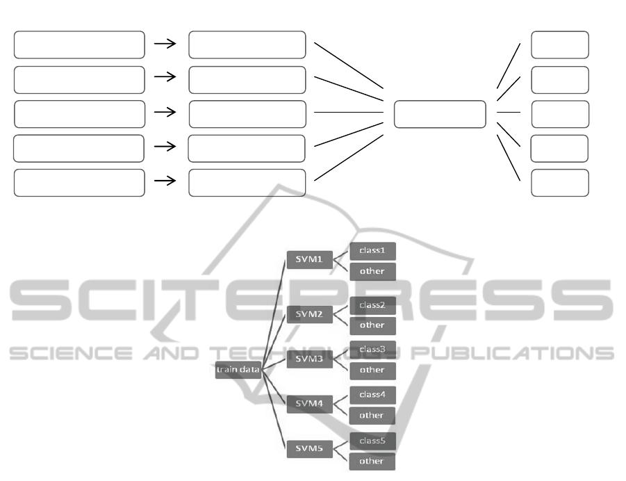
Figure 1: The calculations performed to determine the identity from single-trial in identification mode.
Figure 2: The training and testing manner of SVM network to multiple classifying.
other to contact with data. The separator plate which
has the largest gap from the border plates would be
the best one. SVM, which are non-linear Input
vectors, completed by mapping into a space with
larger dimensions to allow them to be converted to
linear form. And then in this space a linear decision
surfaces are made. Since this mapping feature that
can be said SVM is a general classifying methods
that NN and Polynomial classification are special
cases of it. Another advantage of SVM is that it
won’t be over-trained by training data. SVM in the
general scheme is used for the classifying between
the two classes, and they can also be generalized for
more than two classes by some methods.
2.2.3.1 Proposed SVM Algorithm
There are two basic methods for generalized SVM in
case of multi-class. Classified method, which
separates a class against the remaining classes
(SVM_OAO), and the other that separates a class
against the whole classes. In this paper, a newer
algorithm that actually optimized of the second
method has been used. In this approach in order to
isolate 5 subjects, five SVM networks for training,
were used. The task of each network was separating
the data from other data. This process was conducted
parallel for every five subjects. The architecture of
this method has been shown in figure 2.
And also to test the network, the same structure
was used. Each test data was given to each five
SVM in parallel way, and the output column, which
includes one and zero numbers, is obtained. If the
data of obtained column were all zero, or if there
were more than a one, these states were measured
among wrong or ambiguous answers, in the next
step, the data accuracy of columns which contains
more than a one was reviewed and also the errors of
this stage were gained. Then, drop of the wrong
answers is obtained from the entire first and second
stage, from the total number of given data, the
accuracy rate of the network in classifying was
acquired. In this paper, 50% of the total data has
been used to train. If the amount of training data
were more, we would observe only 1 up to 3 percent
improvement in output. Instead, the training time
1
300×192
2
100×192
3
200×192
4
100×192
5
300×192
EEG Signals PCA Input NN data Classifire
1
300×24
2
100×24
3
200×24
4
100×24
5
300×24
1
2
3
4
5
BIOMETRY BASED ON EEG SIGNALS USING NEURAL NETWORK AND SUPPORT VECTOR MACHINE
377
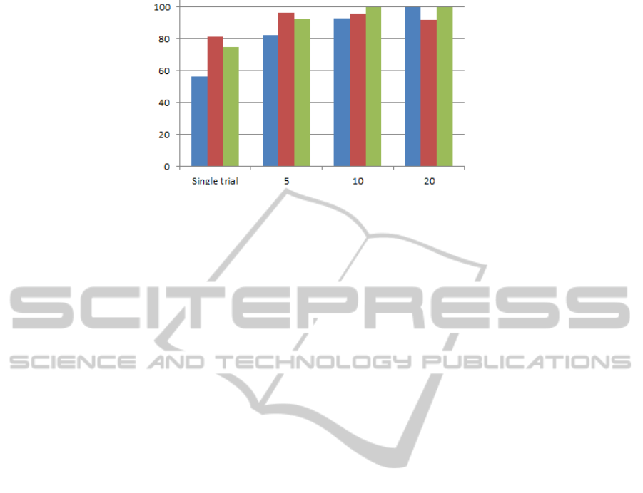
Figure 3: Comparison of results with (Touyama & Hirose, 2008). Green and red are the mean of 10 times applying SVN
and NN respectively. Blue is the results of (Touyama & Hirose, 2008).
was increased and decision network was slowed. For
the best resolution of linear separator, the least
squares method was applied, and RBF Gaussian
function as well kernel function was used. In order
to biometry in identification mode, 50% of total data
sets in order to train the designed SVM network
were given, 50% of remained data was applied to the
designed network model for testing, and output
matrices were obtained.
In verification mode since the only person
claiming must be monitored properly, by using a
SVM separator which only able to separate the two
classes, it can be reviewed the amount of identify on
this base that also shows the results of SVM
method’s feature in pattern recognition. For this
purpose, 10% of signals for every person were
considered as the main data set of verification mode,
and small numbers of different brain signals contain
P300 event were added to verification data set for
stability versus noise, measurement error and non-
target detection. In order to test the network, entire
data was applied to each 5 trained SVM and
accuracy of verification was examined for each
person. To implement these methods, MATLAB
version 7.7 (R2008b) software was used.
3 RESULTS
Achieved results from 10 times performing NN,
applying the whole data set, per verification mode in
order to biometry using a single-trial is recorded in
Table 1. Results of 10 times performing designed
SVM network in verification mode per single-trial
signal are demonstrated in table 2. Results of 10
times performing NN for identification per single-
trial signal and 5, 10 and 20 times averaging have
been illustrated in table 3.Also results of 10 times
performing designed SVM network in identification
mode per single-trial signal and 5, 10 and 20 times
averaging are in table 4. The end columns of all
tables related to 10 times averaging the performing
of networks. Figure 3 shows the comparison of
results with (Touyama & Hirose, 2008).
4 DISCUSSION
According to Table 1, it is observed that acceptable
results have been obtained by the idea of using P300
as a biometric feature in verification mode.
Although there must be more try to achieve better
results, the 72.8% average in correct classification
using NN is successful as first step. The gained
results from tables 1 and 2 also show NN has better
results in comparison with SVM when P300 is not
visible enough. Maximum of results in NN is more
than SVM while the results stability in SVM, per 10
times running the networks, are more than NN.
According to the results shown in table 3, it is
observed that results are increased per five times
averaging, comparison with single-trial mode which
due to signal’s P300 becoming more visible. But
reducing the numbers of training inputs of NN
(which is for decreasing the data set volume in 10
and 20 times averaging in comparison with single-
trial mode and 5 times averaging) is caused
decreasing the percentage of 10 and 20 times
averaging. This means that, the number of samples
for 10 and 20 times averaging was inadequate for
NN. Also it is observed that with even 5 times
averaging we can achieve 100% accuracy in
classification which is the result of using NN.
According to table 4, the results have been improved
by increasing the number of averaging that more
effect of P300 in averaging signal is the cause. It
means that SVM can acceptably save its
performance against small data set volume\. Similar
maximum and averaging amount in each step show
BIOSIGNALS 2012 - International Conference on Bio-inspired Systems and Signal Processing
378

Table 1: The obtained results of 10 times testing the NN by applying the whole data set in single-trial mode per verification
data set due to biometry on verification mode.
1 2 3 4 5 6 7 8 9 10 Max. Mean
72.3 75.3 69.2 71.8 73.8 73.3 74.8 71.5 73 73.3 75.3% 72.8%
Table 2: The obtained results of 10 times testing the SVM by applying the whole data set in single-trial mode per
verification data set due to biometry on verification mode.
1 2 3 4 5 6 7 8 9 10 Max. Mean
57.8 60.7 63.7 61.3 57.8 55.5 54.3 58.3 61.8 60.8 63.7 59.2
Table 3: The results of 10 consecutive running NN in order to identify per single-trial signals and 5, 10 and 20 times
averaging.
Averaging times 1 2 3 4 5 6 7 8 9 10 Max. Mean
0 (single trial) 83.8 81.7 70.8 81 84.7 84.2 80.3 82.2 76.5 86.2 86.2% 81.14%
5 96.7 98.3 99.2 98.3 97.5 97.5 98.3 100 97.5 82.5 100% 96.58%
10 88.3 100 96.7 98.3 96.7 98.3 85 96.7 98.3 100 100% 95.83%
20 90 83.3 93.3 83.3 100 90 96.7 96.7 90 96.7 100% 92%
Table 4: The results of 10 consecutive running SVM in order to identify per single-trial signals and 5, 10 and 20 times
averaging.
Averaging times 1 2 3 4 5 6 7 8 9 10 Max. Mean
0 (single trial) 73 71.6 77.4 78 74.7 75.2 70 75.8 78 76.8 78% 75%
5 93.4 90.6 90.8 89.5 94 92.9 93 93.7 92.7 93.3 94% 92.4%
10 98.7 95 100 97 99.8 97.9 100 100 98.3 100 100% 99.7%
20 100 100 100 100 100 100 100 100 100 100 100% 100%
that similar results have been achieved. According to
the observations, SVM shows more sustainable
results than NN. But 100% results accuracy take
place, only with 5 times averaging in NN. In this
research, for better performance of SVM in high
dimensions if the PCA isn’t used for reducing the
number of features, more favourable results can be
gained. Besides, the obtained NN results, improved
dramatically, since there are no features elimination.
But in this case, the designed network will act very
slowly. Also using PCA to reduce the number of
feature, will makes a more compact database. Using
SVM for the classification due to separation with
maximum margin between two classes makes it
possible that used network has more resistant versus
of noise and additive disturbances. Figure 3
represents significant increases in accuracy
percentage in single-trial mode (81.14%) in
comparison with previous study (56.2%) by using
NN. Also figure 3 shows NN has the best result
when dataset input is enough (single trial and 5
times averaging mode) even P300 is not much clear.
ACKNOWLEDGEMENTS
We thank Mohammad Ravari and Fuad Yahyazadeh
for help with the SVM processing.
REFERENCES
Berger, H., 1938. Das Elektrenkephalogramm des
Menschen, Nova Acta Leopoldina 6. pp 173-309.
Bertillon, A., 1896. Signaletic Instructions including the
theory and practice of Anthropometrical Identifica-
tion. The Werner Company.
Burghardt, B., 2002. Inside iris recognition, Master's
thesis. University of Bristol.
Im, S., Park, H., Kim, Y., Han, S., Kim, S., Kang, C.,
2001. An Biometric Identification System by
extracting Hand Vein Patterns, Journal of the Korean
Physical Society 38, pp. 268-272.
Lindsay, I. & Smith, (2002). A tutorial on principal
components analysis. <http://kybele.psych.cornell.edu
/~edelman/Psych-465Spring-2003/PCA-tutorial>.
Palaniappan, R., 2004. Method of Identifying Individuals
Using VEP Signals and Neural Network. In: IEEE Sci.
Meas. Technol. pp. 16-20
Palaniappan, R., Mandic, D.P., 2005. Energy of Brain
Potentials Evoked During Visual Stimulus: A New
Biometric. In: Int’l Conf. Artificial Neural Network.
pp. 735-740.
Poulos, M., Rangoussi, M., Chrissikopoulos, V.,
Evangelou, A., 1999 Person Identification Based on
Parametric Processing of the EEG. In: IEEE Int’l
Conf. on Electronics Circuits and Systems. Vol. 1, pp.
283-286.
Poulos, M., Rangoussi, M., Chrissikopoulos, V.,
Evangelou, A., 1999. Parametric Person Identification
from the EEG Using Computational Geometry. In
IEEE Int’l Conf. on Electronics Circuits and Systems.
BIOMETRY BASED ON EEG SIGNALS USING NEURAL NETWORK AND SUPPORT VECTOR MACHINE
379

Vol. 2, pp. 1005-1008.
Pierre, M., Nicolas, O., 2010. A Precursor in the History
of Fingermark Detection and Their Potential Use for
Identifying Their Source (1863), Journal of forensic
identification 60, pp. 129-134.
Tangkraingkij, P., Lursinsap, C., Sanguansintukul, S.,
Desudchit, T., 2010. Personal Identification by EEG
Using ICA and Neural Network. Lecture Notes in
Computer Science 6018. Springer Berlin / Heidelberg.
pp. 419-430, 2010.
Touyama, H., Hirose, M. 2008. The Use of Photo
Retrieval for EEG-Based Personal Identification.
Lecture Notes in Computer Science 5068. Springer-
Verlag Berlin /Heidelberg. pp. 276-283
Vogol, F., 1970. The genetic basis of the normal human
EEG, Humangenetik 10. pp.91–114.
Woodward, J. D., Nicholas, Jr., Orlans, M., Higgins, P. T.,
2003, Biometrics. McGraw Hill Osborne. New York.
BIOSIGNALS 2012 - International Conference on Bio-inspired Systems and Signal Processing
380
