EVENT DETECTION USING LOG-LINEAR MODELS FOR

CORONARY CONTRAST AGENT INJECTIONS

Dierck Matern, Alexandru Paul Condurache and Alfred Mertins

Institute for Signal Processing, University of Luebeck, Ratzeburger Allee 160, Lübeck, Germany

Keywords:

Event detection, CRF, MEMM, Graphical modeling.

Abstract:

In this paper, we discuss a method to detect contrast agent injections during Percutaneous Transluminal Coro-

nary Angioplasty that is performed to treat the coronary arteries disease. During this intervention contrast

agent is injected to make the vessels visible under X-rays. We aim to detect the moment the injected contrast

agent reaches the coronary vessels. For this purpose, we use an algorithm based on log-linear models that are

a generalization of Conditional Random Fields and Maximum Entropy Markov Models. We show that this

more generally applicable algorithm performs in this case similar to dedicated methods.

1 INTRODUCTION

Modern surgical treatment is often image supported.

For example, in Percutaneous Transluminal Coronary

Angioplasty (PTCA), cardiac X-ray image sequences

are used in the treatment of the coronary heart dis-

eases. During the intervention, a contrast agent is in-

jected into the vessels to make them visible and en-

able a balloon to be advanced to the place of the lesion

over a guide wire. Contrast agent is given in occa-

sional bursts, thus, the vessels are not constantly visi-

ble. To build a dynamic vessel roadmap (Condurache,

2008) that constantly shows the vessels during the

length of the intervention, we need to detect the mo-

ment the contrast agent reaches the vessels, that is,

the moment they become visible under X-rays. An

algorithm to detect this moment is discussed here.

Dedicated methods for this task can be found in

(Condurache et al., 2004; Condurache and Mertins,

2009). Here we introduce a more general event detec-

tion algorithm based on Log-Linear Models (LLMs)

which is closely related to Conditional Random Fields

(CRFs) (Wallach, 2004; Lafferty et al., 2001) and

Maximum Entropy Markov Models (MEMMs) (Mc-

Callum et al., 2000). Our goal is to show that CRF-

based event detection, as a general framework, is able

to solve event detection problems with accuracy sim-

ilar to or even better than dedicated methods for the

target application.

LLMs, especially CRFs and MEMMs, are ﬁnite

state models (Gupta and Sarawagi, 2005; Wallach,

2004; Lafferty et al., 2001; McCallum et al., 2000)

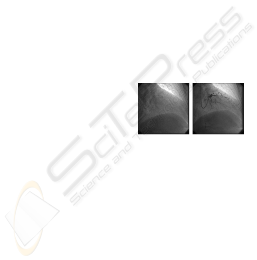
(a) (b)

Figure 1: Two example X-ray images without (a) and with

(b) contrast agent.

which are used for segmentation problems (McCal-

lum et al., 2000; Lafferty et al., 2001). For this task,

an existing, labeled data set is used to train the model.

Then the model is applied to new data sets to generate

a corresponding label sequence. For event detection

problems, the event is usually unknown, thus we have

no labeled data for the events. Therefore, the usual

training algorithms for CRFs (Gupta and Sarawagi,

2005) do not apply. An approach when we have partly

labeled data (Jiao et al., 2006) is not suitable, because

it assumes at least some labels for each class.

MEMMs are Markov models with a maximum en-

tropy approach (McCallum et al., 2000; Gupta and

Sarawagi, 2005). From a graphical point of view,

they are directed models like Hidden Markov Mod-

els (HMMs). If the model is not directed, we have a

(linear chain) CRF. This is important for the applica-

tions: using a MEMM, the probability to observe a

special state depends only on the states before, while

in CRFs, it depends on the states before and after the

172

Matern D., Condurache A. and Mertins A. (2012).

EVENT DETECTION USING LOG-LINEAR MODELS FOR CORONARY CONTRAST AGENT INJECTIONS .

In Proceedings of the 1st International Conference on Pattern Recognition Applications and Methods, pages 172-179

DOI: 10.5220/0003774101720179

 SciTePress

100 200 300

100

150

Frame n

(n) (unfiltered)

100 200 300

100

150

Frame n

y(n) (filtered)

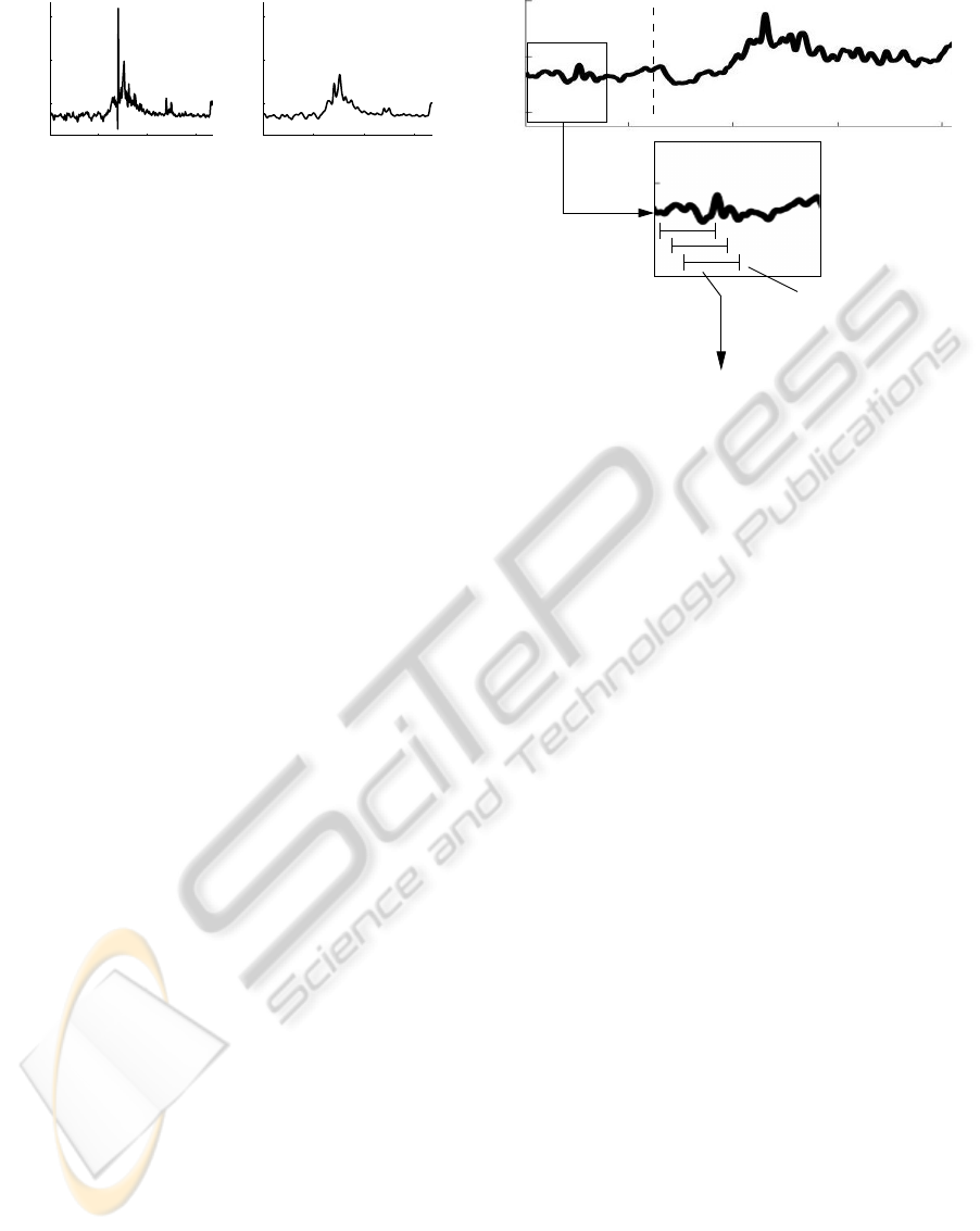
Figure 2: Original vessel feature curve (left hand side) and

the ﬁltered histogram feature curves (right hand side).

actual state. Hence, in MEMMs, we pass forward in-

formation, while in CRFs, the information is passed

forward and backward. This has two important con-

sequences: (i) the usage of CRFs is more accurate

because we use more information for each time step,

and (ii) we cannot apply it for online problems, be-

cause we have to measure the whole data sequence

before the inference. The method we describe here is

a trade of of both approaches. We use several frames

for the inference for a more accurate decision, while

getting only a short and adjustable delay.

We describe a new method to extend the training

algorithm such that we can use an LLM for event de-

tection. We call this the Event Detection Log-Linear

Model (edLLM). This model gives us the opportunity

to conduct the event detection in a more sophisticated

manner, respecting that the normal case may consist

of several characteristics. Furthermore, we introduce

new methods to conduct the inference.

The rest of the paper is structured as follows. In

Section 2, we discuss the features we extract for the

event detection, the model and the test procedure. In

Section 3, we present the results of the experiments.

In Section 4, we give a short conclusion.

2 FEATURE EXTRACTION AND

MODEL DESCRIPTION

From X-ray images, we extract scalar features that

build a feature curve when considering an entire se-

quence. This is afterwards windowed and trans-

formed into a sequence of feature vectors that we use

for event detection. For this purpose, we introduce the

edLLMs, and discuss the training and inference.

2.1 Feature Extraction

From each X-ray image we extract a vessel feature,

sensitive to vessel only. First, a vessel-map showing

contrast-enhanced vessels is computed (Condurache

and Mertins, 2009). Afterwards we compute the the

vessel feature as the 98 percentile of the vessel-map’s

gray level histogram. Because this results in a scalar

Extraction,

normalization

Inference

... ,





x(n − 1)









x(n)









x(n + 1)





, ...

Training

y(n + 1),...,y(n + T )

Figure 3: Schematic representation of the feature extrac-

tion process. Short sequences of the vessel feature curve

are selected, using a sliding window with T − 1 overlap.

From each short sequence y(n + 1),y(n + 2) ..., y(n + T ),

we extract a normalized feature vector x(n). This results in

a sequence of feature vectors, which we analyze with the

edLLM.

value for each frame, for a sequence of X-ray images

this results in a one dimensional sequence of features,

that we call a vessel feature curve. Further, to reduce

noise, an adaptive ﬁlter is applied to this histogram

feature curve. This ﬁlter is deﬁned as follows (Con-

durache et al., 2004; Condurache and Mertins, 2009).

Let y

(n) ∈ R be the unﬁltered vessel feature, then the

ﬁltered vessel feature y(n) is

y(n) := f (n)y

(n) + (1 − f (n))y(n − 1), (1)

f (n) :=



c ∈ [0, 1) if y

(n) − y

(n − 1) ≤ 3

1 otherwise,

where

σ is the estimated standard deviation of the ﬁrst

unﬁltered vessel features. This ﬁlter smoothes only on

stationary intervals. Examples of the unﬁltered and

ﬁltered curves can be seen in Figure 2. A detailed de-

scription how this features are extracted can be found

in (Condurache et al., 2004; Condurache and Mertins,

2009).

2.1.1 Feature Vectors

We analyze the data batch-wise. Each batch consid-

ers several vessel features corresponding to a spe-

ciﬁc portion of the feature curve. This portion is

selected by means of a sliding window of length T

with T − 1 overlap. Therefore, a batch is given by

y(n),y(n + 1),...,y(n + T − 1), one corresponds to

one frame. For each frame we than compute a feature

EVENT DETECTION USING LOG-LINEAR MODELS FOR CORONARY CONTRAST AGENT INJECTIONS

173

vector x(n) that is related to the mean, curvature and

slope in each batch. An ordered set of feature vectors

is a feature vector sequence. A decision is returned

for each feature vector and thus for each frame of the

video sequence, starting at frame T . In the following,

we will discuss the components of the feature vec-

tor by introducing the functions used to compute the

mean, curvature and slope. These features are general

enough to be applicable to many different time series

describe local properties of the vessel feature curve.

A schematic representation of the feature extraction

process can be seen in Figure 3.

We also normalize the feature vectors to reduce

the inﬂuence of outliers. We call a vessel feature out-

lier if it is either very large or small in comparison to

both, the previous and next vessel feature on the fea-

ture curve. The ﬁlter in (1) removes most of the rel-

atively smaller outliers, thus we only need to remove

very large ones.

2.1.1(a) Mean. The ﬁrst two components of the fea-

ture vector are related to the mean of the feature curve.

Let α and β be two scalars with α, β ∈ (0, 1). Then

µ(n+1) := αµ(n) + (1 −α)

∑

T −1

m=0

y(n+m) is a slowly

adapting mean value, and ν(n + 1) := βν(n) + (1 −

β)µ(n) a fast adapting one. We call them “mean val-

ues” because for stationary signals, the adapting mean

values converge to the mean of the signal with in-

creasing T . α and β are adaptation rates and depend

on the frame rate of the analyzed video. Further, let

(m) := y(m) − µ(n) and

(m) := y(m) − ν(n) be

differences to those mean values and a vessel feature.

We want to compare the mean value of a batch to

the adapting mean values. The ﬁrst two components

of the feature vector are

(n) :=





1 −

∑

T −1

m=0

(m + n)

2 · T ·





· 10,

(n) :=





1 −

∑

T −1

m=0

(m + n)

5 · T ·





· 10,

where

is the estimated variance of the training

data. These functions are positive if the mean of the

batch is close to the adapting mean values, and neg-

ative otherwise. The scaling within the roots control

what we call “close”. The factor 10 is to emphasize

these features, because they act in a manner similar

to the statistical test used in (Condurache et al., 2004;

Condurache and Mertins, 2009).

2.1.1(b) Curvature. We extract features related to the

curvature. These features are computed as the differ-

ence of each element of a batch to the mean of a batch.

The next T components of the feature vector are:

2+k+1

(n) := y(n + k) −

T −1

∑

m=0

y(n + m),

for k = 0,1,2,...,T − 1.

2.1.1(c) Slope. The last L components of the

feature vectors are used to measure the slope of

a batch. We deﬁne the slope of a batch as

the slope of its linear regression, that is

b(n) :=

arg min

b∈R

∑

T −1

m=0

(y(n + m) − y(n) − b · m)

For each batch, we compare these slopes to a set

of L sample slopes. Let b

min

be the minimal slope that

is observed in the training batches, and b

max

the max-

imal slope. Then a sample slope w

, l = 1,2,...,L, is

deﬁned as w

L−l

L−1

min

l−1

L−1

max

. The function we

use to compare slopes of batches to the sample slopes

2+T +l

(n) := 1 −

b(n) − w

l+1

− w

for l = 1,2,...,L. This function is positive if a new

slope is close to the respective sample slope, and neg-

ative else.

2.1.1(d) Outliers. For each batch y(n),y(n +

1),...,y(n + T − 1), we have deﬁned a vector ξ(n) :=

[ξ

(n)]

i=1

with N = 2 + T + L. The functions

,ξ

,...,ξ

describe properties of each batch, but

are affected by outliers. Let v(n) :=

∑

T −1

m=1

(y(n +m)−

y(n + m − 1))

be the (unnormalized) local variation.

Then, the normalized outlier-robust feature vector is

x(n) :=

v(n)

ξ(n). We call x(n) the feature vector at

lag n.

This local variation increases in the presence of

large outliers. This normalization does not remove

the possibility to detect events in the feature vector

sequence, because we assume that any real event is

visible for several successive frames.

2.2 Event Detection Log-linear Model

In the last section, we have described the how to gen-

erate the feature vector sequence x. In this section, we

describe the edLLM in detail. We ﬁrst introduce the

edLLM in Section 2.2.1 and describe the training and

inference afterwards.

2.2.1 Model Description

We propose a LLM that is specialized on event de-

tection. These models process sequences of data in a

ICPRAM 2012 - International Conference on Pattern Recognition Applications and Methods

174

manner similar to CRFs and MEMMs. The sequence

we use here is the sequence of feature vectors.

Let x with x(n) ∈ R

be a feature vector se-

quence and s a corresponding state sequence, with

s(n) ∈ {ζ

,ζ

,...,ζ

}. We use the convention that

the states ζ

,ζ

,...,ζ

describe the normal case, and

the event, that is in our case the occurrence of the

contrast agent. The training data includes no events:

s(n) 6= ζ

. Using several states for the normal case,

we obtain a highly descriptive model that covers the

various cases of what is deﬁned to be normal.

For our purpose, we need now to link the training

data to the states of the normal case. This is an unsu-

pervised classiﬁcation problem, as we need to assign

each feature vector from the training data one label

from the set {ζ

,ζ

,...,ζ

}. Let y

min

be the mini-

mum vessel feature in the training data and y

max

the maximum one. We deﬁne a

K−q+1

min

+(1 −

K−q+1

max

for q = 1, 2, . . . , K + 1, and we label the

training data by s(n) = ζ

if a

≤

∑

T −1

m=0

y(n + m) <

q+1

The idea of the edLLM is to label a feature-vector

sequence of a certain length at once. As each feature

vector is computed from a batch of vessel features, we

use then a larger context for improved decision. We

determine the probability of a state sequence, given a

sequence of feature vectors, similar to CRFs (Gupta

and Sarawagi, 2005). As a difference to CRFs, we

work with sequences of feature vectors, that we deﬁne

with the help of a sliding window. Thus we can use

this algorithm online. For the training, however, we

use the whole training data in a single sequence of

feature vectors. he training is conducted in the same

way as for CRFs and MEMMs, except for the penalty

term as described in Section 2.2.2.

2.2.1(a) Log-linear model. Let M ∈ N be the length

of a feature vector sequence x

and t

∈ N

be a

starting index of this sequence, i = 0,1,... where

i = 0 denotes the training data. For a shorter notation,

let x

:= [x(t

+ m)]

m=1

. We do the same with the

states: s

(m) := s(t

+ m) and s

:= [s

(m)]

m=1

. The

probability of s

, given x

and s

(0) is deﬁned by

(Gupta and Sarawagi, 2005)

p(s

(0)) :=

exp



∑

m=1

Φ(s

(m − 1), s

(m),x

,m)



Z(x

)

. (2)

Z(x

) is a normalization value such that p(s

(0))

is a probability. λ is a weighting vector that identiﬁes

features that are important for a successful description

of the normal case. The function Φ establishes the re-

lationship between the feature vectors and the states.

It is deﬁned by

Φ(s

,n) :=







(n) · [[s

= ζ

]]]

k=1

[[[s

= ζ

]] · [[s

= ζ

]]]

j=1

k=1

(n) · [[s

= ζ

]]







. (3)

with x

(n) ∈ R

, Φ(s

,n) ∈ R

(N+1)K+K

. [[P]] =

1 if the predicate P is true and 0 otherwise (Gupta

and Sarawagi, 2005). For each sequence i, we need

an initial label s

(0) = s(t

). For the training data

(that is, i = 0), we have no information about s

(0) =

s(0), so we use an arbitrary symbol such that s(0) /∈

{ζ

,ζ

,...,ζ

} (Gupta and Sarawagi, 2005). For

i = 1, the initial label is s

(0) = s(t

). This is one of

the labels used for the training. For i > 1, s

(0) = s(t

)

is determined by the inference at this time step.

2.2.1(b) Example. Assume we have only 2D fea-

ture vectors (N = 2) and a sequence of length M = 2

for some i with i > 1, x

(1) = [a,b]

and x

(2) =

[c,d]

. Further, assume we have K = 2, that is,

(n) ∈ {ζ

,ζ

}, n = 1,2. Note that with this pa-

rameters, (K + 1)

= 9 sequences are possible. We

assume that the ﬁrst label is ζ

, and then we build our

example for all possible length 2 sequences.

Using the deﬁnitions above, Φ(ζ

,ζ

,1) =

[a,b,0,0,0,0,0,0,0,0]

, and Φ(ζ

,ζ

,2) =

[c,d, 0, 0, 1, 0, 0, 0, 0, 0]

. The ﬁfth entry of

Φ(ζ

,ζ

,1) indicates the “transition” from state ζ

to ζ

(the systems stays in state 1). The ﬁrst two en-

tries are x

(1). If we use the state sequence [ζ

,ζ

]

then Φ(ζ

,ζ

,2) = [0,0,c,d,0,1,0,0,0,0]

so the third and fourth entry of Φ(ζ

,ζ

,1)

are x

(2). The sixth entry of Φ(ζ

,ζ

,1) is

1, due to the transition from ζ

to ζ

. If we as-

sume an event at lag two, that is s(2) = ζ

, then

Φ(ζ

,ζ

,2) = [0, 0, 0, 0, 0, 0, 0, 0, c, d]

We further assume that the weighting vector is

λ = [λ( j)]

j=1

] = [1, −1, −1, 1, 1, 0.5, 0.5, 1, 1, 1]

Then, according to Equation (2), we compute the

unnormalized probability as

˜p(s|x

,s(0)) =

exp

∑

m=1

Φ(s(m − 1), s(m), x

,m)

. (4)

s(0) is some arbitrary symbol such that

s(0) /∈ {ζ

,ζ

}. Hence, ˜p([ζ

,ζ

]

,s(0)) =

exp(λ

Φ(ζ

,ζ

,s(0))) = exp(a − b + c − d + 1) =

EVENT DETECTION USING LOG-LINEAR MODELS FOR CORONARY CONTRAST AGENT INJECTIONS

175

exp(a − b) · exp(c − d + 1). For the second ex-

ample sequence, ˜p([ζ

,ζ

]

,s(0)) = exp(a −

b + d − c + 0.5) = exp(a − b) · exp(d − c + 0.5).

The unnormalized probability of an event at lag

two is ˜p([ζ

,ζ

]

,s(0)) = exp(a − b + c + d) =

exp(a − b) · exp(c + d).

Now we want to decide which of these state se-

quences provides the highest probability. If c >

d − 0.25 and d < 0.5, the most probable sequence is

[ζ

,ζ

]

. If c < d − 0.25 and 0.25 > c, it is [ζ

,ζ

]

otherwise, it is [ζ

,ζ

]

. In this case, we have ob-

served an event at lag two. Note that these limits de-

pend on the weighting vector λ which includes a scal-

ing.

In this example, we can interpret λ as follows.

The ﬁrst N = 2 entries of λ describe the state ζ

that means, a positive value “prefers” a corresponding

positive value in x

(if an entry in λ is positive and the

corresponding one in x

too, the probability for this

state is higher than otherwise), a negative in λ a neg-

ative one in x

; a zero in λ can be interpreted as “no

inﬂuence” on the probability. The next N entries de-

scribe the state ζ

. The next K

= 4 entries describe

the transition probabilities between the normal case

states. The last N entries describe the event.

2.2.2 Parameter Estimation

The weighting vector λ is estimated in the training

phase. During training, we maximize p(s

,s(0))

(see Equation (2)) with respect to λ, given the train-

ing data and a corresponding state sequence, where

is the training data and s

the corresponding label

sequence.

Let t

be the start index of the training data (i.e.,

= 0) and M

the number of training feature vectors.

Then, we obtain

Φ(s

) :=

∑

m=1

Φ(s

(m − 1), s

(m),x

,m).

In the training phase, we optimize L

, the pe-

nalized log-likelihood of p(s

,s(0)) (Gupta and

Sarawagi, 2005), deﬁned as

:= log(p(s

,s(0))) − F(λ)

= λ

Φ(s

) − log Z(x

) − F(λ), (5)

where F(λ) :=

||Dλ||

−

λ with

e := [ ˜e

]

(N+1)K+K

k=1

and

˜e







∑

i=1

[[s(i) 6= ζ

]] if ( j − 1) · N < k ≤ j · N,

0 otherwise.

F(λ) is the penalty term. It is necessary for two

purposes: to avoid overﬁtting (Gupta and Sarawagi,

2005), and to adapt the training to our event detection

setup. For the former purpose,

e compensates the dif-

ferent numbers of training vectors for each state. For

the latter purpose, we deﬁne the penalty matrix D by

D := [D(i, j)]

(N+1)K+K

i, j=1

with

D(i, j) :=











1 if i = j, i, j ≤ N · K + K

2N+1

if i = j, i, j > N · K + K

2N+1

if i 6= j, i, j > N · K + K

if i = k · j + N · K + K

k = 1,2,...,K,

0 otherwise.

We use this penalty matrix in contrast to how training

is conducted for usual LLMs (Gupta and Sarawagi,

2005; Lafferty et al., 2001) because we assume that

we cannot train for ζ

in a direct manner, as the

training data x

does not include any events, that is

(m) 6= ζ

, m = 1, 2, . . . , M

Because we want to determine λ such that the

penalized log-likelihood (see Equation (5)) is maxi-

mized, the training of the edLLM is an optimization

problem. The gradient of the penalized log-likelihood

∇L

= Φ(s

) − E(s|x

,λ) − Dλ +

where E(s|x

,λ) is the expected value of the sequence

s, given x

and λ. An efﬁcient algorithm to com-

pute E(s|x

,λ) can be found in (Gupta and Sarawagi,

2005). The training processes in several iterations. At

iteration τ, λ is updated by λ

(τ+1)

:= λ

(τ)

+0.3·∇L

(τ)

The constant 0.3 in the update of λ is selected empir-

ically.

2.2.3 Inference

With a trained model, we want to determine the prob-

ability of a state sequence for a new feature vector se-

quence. For the event detection, the most interesting

task is to measure the probability to detect an event,

that is the probability that the state ζ

, appears in a

feature vector sequence.

As described before, i > 0 indicate the i-th feature

vector sequence of length M that we want to analyze,

with t

as its starting index. We analyze the whole se-

quence of feature vectors x batchwise to increase our

classiﬁcation results. These feature vector sequences

do overlap by d vectors, because with d > 0, we

increase the classiﬁcation results of later feature vec-

tor in each feature vector sequence x

. Because each

feature vector corresponds to a frame of the X-ray im-

ages, d is actually a delay. We also can set d = 0 if

we cannot accept one, with costs of precision.

For each feature vector sequence x

, we ﬁrst want

to estimate a state sequence s

. An exhaustive search

ICPRAM 2012 - International Conference on Pattern Recognition Applications and Methods

176

for each possible state sequence corresponding to this

feature vector sequence is not feasible, because we

would have to test (K + 1)

different state sequences.

To circumvent this problem, we deﬁne a forward path

i,m

and a backward path β

i,m

(Gupta and Sarawagi,

2005) recursively by

i,m

(k) :=

∑

j=0

i,m−1

( j) · exp(λ

Φ(ζ

,ζ

,m)),

and

i,m

( j) :=

∑

k=0

i,m+1

(k) · exp(λ

Φ(ζ

,ζ

,m + 1)),

where m = 1, 2, . . . , M, Z

and Z

are constants such

that

∑

j=1

i,m

( j) =

∑

k=1

i,m

(k) = 1. α

i,m

(k) is the

probability that we observe ζ

at lag m in the feature

vector sequence x

, given the previous states, β

i,m

( j)

is the probability of state ζ

at lag m in the feature

vector sequence x

, given the following states. The

probability of state ζ

at time step m in x

is given by

p(s

(m) = ζ

) :=

i,m

( j) · β

i,m

( j)

α,β

, (6)

where Z

α,β

is a normalization constant such that

p(s

(m) = ζ

) is a probability.

We use this forward-backward-algorithm to max-

imize the information we use for labeling, and there-

fore the reliability of the method. For the same pur-

pose, we also do not apply the inference of the feature

vector sequences independently. For the ﬁrst feature

vectors of the sequence x

i+1

, we pass forward infor-

mation from x

which we have labeled before.

Assume we have calculated α

i,m

(k) and β

i,m

( j),

j, k = 1, 2, . . . , K. To initialize the inference on

the next feature vector sequence x

i+1

, we de-

ﬁne the forward path initiation by α

i+1,0

(k) :=

p(s

(M − d) = ζ

) and the backward path initiation

as β

i+1,M+1

( j) :=

K+1

. Now we can conduct the in-

ference on the feature vector sequence x

and use the

feature vectors of the sequences before without a new

labeling.

In the case of event detection, we are particularly

interested in the probability of the event state ζ

, that

is p(s

(m) = ζ

) (see Equation (6)). We can assume

that we have detected an event if p(s

(m) = ζ

) > θ

for some 0 < θ < 1. However, this method is very

sensitive to noise in the probability of the event state,

which can occur if the number of training feature vec-

tors is limited or the variation in the data is high. A

noise-robust method is discussed next.

...

Training Inference

x: ...

Figure 4: We apply the inference on short sequences of fea-

ture vectors, each of length M. These intervals overlap with

d feature vectors. Hence, d vectors are re-labeled, using

more feature vectors and therefore more information. The

ﬁrst feature vector sequence x

is initialized to include sev-

eral features that belong to the training set.

2.2.3(a) CUSUM test. The probability for the obser-

vation of the event state ζ

in a feature vector se-

quence x

at lag m is p(s

(m) = ζ

). We need an

interpretation of this probability. We use a Cumu-

lated Sum (CUSUM) test (Basseeville and Nikiforov,

1993) to decide if an event has occurred. For this pur-

pose, we deﬁne c(m) with

c(m) := c(m − 1) + p (s

(m) = ζ

) − c

where c

is estimated such that c(m) ≤ 1 for m ≤ M

that is, we detect no event in the training data. An

event has occurred if c(m) > 1. We set c(m) to zero

either if an event has occurred or if c(m) ≤ 0.

3 EXPERIMENTS, RESULTS AND

DISCUSSION

We test our algorithm on the same X-ray image se-

quences used in (Condurache et al., 2004). Some ex-

amples are shown in Figure 1, and the vessel feature

curves in Figures 2 and 5.

For an event detection algorithm, the data provides

several interesting properties that make it challenging

and representative for other event detection problems.

First, it is generated by real measurements, no simu-

lation. Second, the state of the coronary arteries de-

pends on the heart beat, so a periodicity can be as-

sumed. Without it training could not be applied, be-

cause training data does not explain the normal case

in the inference. Further, the data depends on machine

settings and human interaction, so each sequence can

have very different statistical properties which are, in

EVENT DETECTION USING LOG-LINEAR MODELS FOR CORONARY CONTRAST AGENT INJECTIONS

177

fact, unknown. Our algorithm is a more general event

detection algorithm which can successfully analyze

very different time series.

We test the algorithm on nine different sequences

of vessel features. To evaluate our results we use the

same manual ground-truth proposed in (Condurache

et al., 2004). Note that this manual ground-truth is in-

ﬂuenced by the quality of the X-ray images, the pre-

cise index of the frame where the contrast agent be-

comes visible is afﬂicted by small errors. Hence, we

rate the experiment as a success if the detection is be-

low 12 frames to the manual ground truth, that is one

second.

Because the data is measured in a surgical treat-

ment, the number is limited. To design the features,

we randomly have chosen three of the sequences, and

the tests are conducted on all nine sequences. As

discussed in 2.1, we use a sliding window of length

T = 36. We produce N = 41 dimensional feature

vector sequences, with L = 3 sample slopes w

. For

each of these feature vectors sequences, we train an

edLLM with K = 5 on the ﬁrst M

= 64 feature vec-

tors. Therefore, the training sequence are the ﬁrst 99

ﬁltered histogram features (8.25 seconds). We tested

different numbers of feature vectors for the inference.

With M = 10 and a delay d = 2, we obtain the best re-

sults. Our method is robust with respect to the choice

of these parameters.

Our method is robust with respect to the choice of

these parameters. We have tested different parameters

(L from 3 to 9, T from 10 to 50) without noting any

signiﬁcant change in the obtained results.

Our features are well suited to analyze curves such

as the vessel feature curve. Besides mean, curva-

ture and slope, we have also tested other features like

skewness or a direct quantization of the features and

obtained worse results. The feature vectors that are

introduced in Section 2.1.1 are effective for the event

detection. Not every component of the feature vec-

tors have the same inﬂuence on the results for every

sequence, but we could not reduce the feature vec-

tors without decreasing the results for at least one se-

quence.

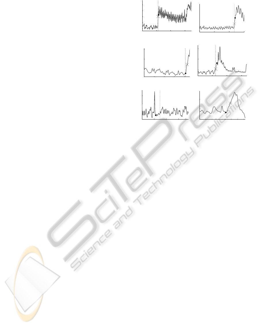
In Figure 5, we can see several detection results.

Displayed are the manually labeled critical point and

the messured one, with both the algorithm proposed

in (Condurache et al., 2004) and the new proposal.

In six of the nine experiments, the automatically

detected events are below 12 frames (below one sec-

ond) to the manually ones, in two experiments the

events are detected too soon. Those two sequences

are contaminated by noise to such an amount that nei-

ther the adaptive ﬁlter nor our feature extraction can

deal with it.

200 400 600

event − estimated event: −6

dedicated method: 1

100 200 300

100

120

140

160

event − estimated event: −5

dedicated method: 0

50 100 150 200

100

event − estimated event: −1

dedicated method: −9

100 200 300

event − estimated event: −9

dedicated method: 0

100 200 300

event − estimated event: 35

dedicated method: not detected

20 40 60 80 100 120 140

100

event − estimated event: 4

dedicated method: −10

Figure 5: Several sequences of coronary contrast agent in-

jections: the vessel features (dark gray curve), the manually

selected critical point (dashed gray line), the detected event

(black dot) and the method provided in (Condurache et al.,

2004) (black cross) For the last test, the training for the nor-

mal case has been reduced to 60 frames because the contrast

agent has been injected too early.

4 SUMMARY AND

CONCLUSIONS

We have described an event detection method and ap-

plied it on the detection coronary contrast agent injec-

tions. The results are comparable or even better than

the dedicated method (Condurache et al., 2004; Con-

durache and Mertins, 2009; Condurache, 2008). Due

to the decision to analyze batches of frames rather

than each frame independently, it is not possible to

detect the contrast agent immediately, but after a few

frames, however, this lateness is below the human re-

action time. Further, we describe a general method

able to detect arbitrary events, not just the occurrence

of the contrast agent.

The edLLM is more adaptable than the dedicated

method. For example, it is not limited to the features

we use in Section 2.1. The training implicitly includes

a selection of good features, so the set of features

can be increased and adapted to more speciﬁc or even

totally different problems. The features we used in

this paper can be interpreted as a starting point: they

are general applicable and explain short sequences of

curves. More specialized features can be adapted, the

training or inference does not have to be altered.

ICPRAM 2012 - International Conference on Pattern Recognition Applications and Methods

178

The delay d we include in our algorithm is used to

increase the precision of our labeling and is chosen

such that the classiﬁcation is almost instantaneous.

Setting d = 0 eliminates the delay, bud decreases the

precision with which an event is detected. However,

this does not necessary afﬂict the detection of events

itself.

If we compare the edLLM to CRFs and MEMMs

from a theoretical point of view, we see a lot of sim-

ilarities. In fact, we can create a CRF and a MEMM

for the event detection by altering the length of the

window of feature vectors M and the delay d in the

inference. If M is equal to the whole sequence of fea-

ture vectors and d = 0, we have a CRF, that is, the

state sequence can be represented by an undirected

graph. If M = 1 and d = 0, we consider a MEMM. By

adapting the functions for the feature vectors and the

labeling for the training, we can adapt this method for

many other event detection problems, even to ofﬂine

problems using CRFs and online problems where we

can not accept a delay, using MEMMs.

REFERENCES

Basseeville, M. and Nikiforov, I. V. (1993). Detection of

Abrupt Changes: Theory and Application, page 35ff.

Prentice-Hall.

Condurache, A., Aach, T., Eck, K., and Bredno, J. (2004).

Fast Detection and Processing of Arbitrary Contrast

Agent Injections in Coronary Angiography and Fluo-

roscopy. In Bildverarbeitung für die Medizin (Algo-

rithmen, Systeme, Anwendungen), pages 5–9.

Condurache, A. P. (2008). Cardiovascular Biomedical

Image Analysis: Methods and Applications. GCA-

Verlag, Waabs, Germany. ISBN 978-3-89863-236-2.

Condurache, A. P. and Mertins, A. (2009). A point-event

detection algorithm for the analysis of contrast bolus

in ﬂuoroscopic images of the coronary arteries. In

Proc. EUSIPCO 2009, pages 2337–2341, Glasgow.

Gupta, R. and Sarawagi, S. (2005). Conditional Random

Fields. Technical report, KReSIT, IIT Bombay.

Jiao, F., Wang, S., Lee, C.-H., Greiner, R., and Schuurmans,

D. (2006). Semi-supervised conditional random ﬁelds

for improved sequence segmentation and labeling. In

Proceedings of the 21st International Conference on

Computational Linguistics and the 44th annual meet-

ing of the Association for Computational Linguistics,

ACL-44, pages 209–216, Stroudsburg, PA, USA. As-

sociation for Computational Linguistics.

Lafferty, J. D., Mccallum, A., and Pereira, F. C. N. (2001).

Conditional random ﬁelds: Probabilistic models for

segmenting and labeling sequence data. In ICML ’01:

Proceedings of the Eighteenth International Confer-

ence on Machine Learning, pages 282–289, San Fran-

cisco, CA, USA. Morgan Kaufmann Publishers Inc.

McCallum, A., Freitag, D., and Pereira, F. C. N. (2000).

Maximum entropy Markov models for information

extraction and segmentation. In ICML, pages 591–

598.

Wallach, H. M. (2004). Conditional Random Fields: An

introduction. CIS Technical Report MS-CIS-04-21,

University of Pensilvania.

EVENT DETECTION USING LOG-LINEAR MODELS FOR CORONARY CONTRAST AGENT INJECTIONS

179