A GENERAL ALGORITHM FOR CALCULATING FORCE

HISTOGRAMS USING VECTOR DATA

Daniel Recoskie, Tao Xu and Pascal Matsakis

School of Computer Science, University of Guelph, Guelph, Ontario, Canada

Keywords: Relative position descriptors, Shape descriptors, Polygonal objects.

Abstract: The histogram of forces is a generic relative position descriptor with remarkable properties, and it has found

many applications, in various domains. So far, however, the applications involve objects in raster form. The

fact is that several general algorithms for the computation of force histograms when dealing with such

objects have been developed; on the other hand, there is no general algorithm available for objects in vector

form, and the algorithms for raster objects cannot be adapted to vector objects. Here, the first general

algorithm for calculating force histograms using vector data is presented.

1 INTRODUCTION

The histogram of forces is a generic relative position

descriptor with high discriminative power and

remarkable properties. It was introduced by Matsakis

and Wendling (1999) with the aim of developing

new models of directional relations (such as right,

left, above, below) between 2-D objects. The spatial

organization of 2-D objects is a subject of interest in

many disciplines (e.g., computer science, cognitive

science, linguistics, geography), with applications in

various domains (e.g., medical imaging, robot navi-

gation, content-based image retrieval, geographic

information systems). The histogram of forces has

been used, e.g., in a geospatial information retrieval

and indexing system (Shyu et al., 2007); for scene

matching (Sjahputera and Keller, 2007); to interpret

human-to-robot commands and generate robot-to-

human feedback (Skubic et al., 2004); along with a

land cover classification system (Vaduva et al., 2010).

Many other applications are mentioned in a recent

paper by Matsakis et al. (2011): the classification of

skull orbits and sinuses; the recognition of graphical

symbols in technical line drawings; the translation of

hand-sketched route maps into linguistic descrip-

tions; etc. The above-mentioned applications deal

with 2-D objects in raster form. These objects can be

crisp or fuzzy, connected or disconnected, with or

without holes, disjoint or overlapping. The fact is

that several general algorithms for the computation

of force histograms when dealing with such objects

have been developed. The traditional algorithm

(Matsakis and Wendling, 1999) runs in O (Kk

√

time, where K is the number of directions in which

forces are considered, k is the number of nonzero

membership degrees and N is the number of pixels

in the image. A variant runs in O (KkN

√

N) time.

Another runs in O (KN

√

N) (Wang et al., 2004). A

completely different algorithm is in O (N logN) (Ni

and Matsakis, 2010). Which algorithm or variant

performs better under which conditions is an issue

discussed by Ni and Matsakis (2010). As these

authors acknowledge, however, the algorithms

above cannot be adapted to objects in vector form,

and there is no general algorithm for the compu-

tation of force histograms in the case of vector

objects (Matsakis et al., 2011). The present paper

fills this important lacuna. The concept of the

histogram of forces is described in Section 2. The

new algorithm is introduced in Section 3.

Experimental results follow in Section 4, and

Section 5 concludes the paper.

2 BACKGROUND

2.1 Objects

Consider a fuzzy subset A of the Euclidean plane.

Every point p of the plane has therefore a grade of

Recoskie D., Xu T. and Matsakis P. (2012).

A GENERAL ALGORITHM FOR CALCULATING FORCE HISTOGRAMS USING VECTOR DATA.

In Proceedings of the 1st International Conference on Pattern Recognition Applications and Methods, pages 86-92

DOI: 10.5220/0003781600860092

 SciTePress

membership in A. This grade, A(p), is 0 if p does not

belong to A at all; it is 1 if p totally belongs to A; it is

a value between 0 and 1 otherwise, and the greater

A(p) the more p belongs to A. The α-cut of A, where

0<α≤1, is the (crisp, ordinary) set of points p such

that A(p)≥α. In this paper, an object is a fuzzy subset

A of the Euclidean plane such that any A(p) belongs

to the set {α

,α

,…,α

k+1

}, with 1=α

>α

>…>α

k+1

=0,

and the intersection between any α

-cut of A and any

straight line has a finite number of connected

components.

2.2 Force Histograms

Consider two distinct infinitesimal particles p and q

of mass m and n. According to Newton’s law of

gravity, p exerts on q the force

mn / | |

, (1)

where

→

is the vector from q to p and |

→

| its

length. This force tends to move q towards p, and its

magnitude is mn / |

→

. Now, consider two objects

A and B. They can be seen as flat metal plates of

constant and negligible thickness: the area mass

density of A at point p is the grade of membership

A(p), and the area mass density of B at q is B(q).

Every point p of A exerts on every q≠p of B an

infinitesimal gravitational force, and the vector sum

of all these forces, i.e., the resultant force exerted by

A on B, can be found using integral calculus.

Instead, consider a real number r and a direction θ,

replace (1) with (2), or with (3), and calculate the

magnitude

(θ) of the vector sum of all the

infinitesimal forces in direction θ (Fig. 1). The

function

so defined is called a force histogram.

It is one possible representation of the position of A

relative to B.

mn / | |

r+1

(2)

min{m, n}/ ||

(3)

Figure 1: Every point of A exerts on every point of B an

infinitesimal force. Using integral calculus, find the vector

sum of the forces in direction θ. Its magnitude is

(θ)

2.3 Properties

The interest in force histograms lies in the fact that

they are relative position descriptors with high

discriminative power and remarkable properties.

Consider a real number r and two objects A and

B. Equation (4) holds for any θ.

(4)

Let rot be a ρ-angle rotation and let sca be a uniform

scaling with positive scale factor λ. The force

histograms

rot (A) rot (B)

and ϕ

sca( A) sca(B)

can be

expressed in terms of

. Equations (5) and (6)

hold for any θ.

(5)

(6)

Actually, any

aff (A) aff (B)

, where aff denotes an

invertible affine transformation, can be expressed in

terms of

. See (Matsakis et al., 2011) (Ni and

Matsakis, 2010) for details. Note that the grade of

membership of a point p in the object aff(A) is, by

definition, aff(A)(p)=A(aff

−1

(p)); likewise,

aff(B)(p)= B(aff

−1

(p)). Now, let A

denote the α

-cut

of A and let B

denote the α

-cut of B. If the forces

are as in (2), then (7) holds; and if they are as in (3),

then (8) holds.

(7)

(8)

Assume A and B are crisp, i.e., all grades of

membership are in {0,1}. Consider a tuple (A

, A

…, A

) of crisp objects, where a is a positive integer.

Assume the interior of A

∩ A

is empty for any i≠j

and the closure of A is equal to the closure of ∪

We then say that (A

, A

, ..., A

) is a partition of A.

Likewise, assume (B

, B

, ..., B

) is a partition of B.

Equation (9) holds for any θ.

(9)

r has an interesting impact on the histogram. When r

is zero,

responds equally to changes in the

closest parts and in the farthest parts of A and B.

When r< 0, it responds more to changes in the

farthest parts, and the greater | r | the more

asymmetric the response. When r > 0, it responds

more to changes in the closest parts; so much so that

the histogram values are infinite if, e.g., r ≥1 and the

objects overlap (i.e., the interior of their intersection

is not empty). Finally, note that the relative position

descriptor

becomes a powerful shape descript-

→

(θ) =ϕ

(θ+π)

rot (A) rot(B)

(θ) =ϕ

(θ−ρ)

(

)

(

)

(

)

3−

(θ)

(θ) = (α

−

j=1

∑

i=1

∑

i+1

)(α

−α

j+1

) ϕ

(θ)

(

)

(

−

i+1

)

(θ)

i=1

∑

(θ) =ϕ

(θ)

j=1

∑

i=1

∑

A GENERAL ALGORITHM FOR CALCULATING FORCE HISTOGRAMS USING VECTOR DATA

(a) (b) (c)

Figure 2: Partitioning of the objects. (a) Each object is divided into trapezoidal pieces. Note that A and B are not necessarily

convex or disjoint: there may be more than two pieces between two consecutive lines, and some pieces may intersect. (b)

The trapezoids p

and q

are cut along the dotted lines into three pieces each. (c) p

is broken into p

and q

, and q

is broken into q

and p

(a) (b) (c) (d)

Figure 3: Two trapezoids A

and B

between two consecutive lines. There are 4 cases. Note that in (a), the trapezoids may

share one vertex or one edge; in (b) they may only share one vertex.

tor when r<1 and the two objects A and B are equal

(Matsakis et al., 2011).

3 ALGORITHM

3.1 Vector Objects

In the remainder of this paper, we assume that every

-cut of an object can be expressed using the union

and difference set operations in terms of a finite

number of simple polygons

, …, where

the edges of

and

do not intersect if u≠v.

Note that an object may be crisp or fuzzy, convex or

concave, connected or disconnected, and may have

holes in it. Practically, each object is described in a

text file as the list of its cuts (sorted by increasing

); each cut is described as a set of polygons (in any

order); each polygon as a list of vertices (listed either

clockwise or counterclockwise); each vertex as a pair

of coordinates

x and y.

3.2 Handling of Vector Objects

As per (7) and (8), the handling of any two objects

comes down to the handling of crisp objects. Let us

explain, therefore, how to calculate

(θ) when A

and B are crisp. First, a partition (A

) of A and a

partition (

) of B are obtained as follows. The

straight lines in direction θ that pass through the

objects’ vertices divide the objects into trapezoidal

(or triangular) pieces (Fig. 2

a). Consider a piece of A

and a piece of

B between two consecutive lines. If

two nonparallel edges of these pieces intersect, an

additional line in direction θ is drawn through the

intersection point. This line divides the two pieces

into smaller pieces (Fig. 2

b). Consider two of these

smaller pieces, between two consecutive lines. If an

edge of the piece of

A runs inside the piece of B, or

vice versa, both pieces are broken into even smaller

pieces (Fig. 2

c). The partitioning is then complete,

and

(θ) can be calculated as in (9). Note that

(θ)

= 0 unless A

and B

are between two

consecutive lines. If they are, 4 cases must be

considered (Fig. 3): in each case,

(θ)

can be

expressed in terms of r, θ, ε, x

, x

, y

, z

where

, x

, z

are edge lengths and ε, y

, y

are

distances between edges (Fig. 4). These expressions

result from the calculation of triple integrals, and are

given in Table 2. The functions

, f

are as in

Table 1, and

t(θ) =

max{ cos(θ) ,sin(θ) }

4 EXPERIMENTS

The general algorithm for force histogram calculation

ICPRAM 2012 - International Conference on Pattern Recognition Applications and Methods

Figure 4:

(θ)

can be expressed in terms of r, θ, ε, x

, x

, y

, z

. See Table 2. Note that the vertices of A

and Bj

are projected onto horizontal lines if

cos(θ) > sin(θ)

and onto vertical lines otherwise.

Table 1: The functions f

, f

(x, y) f

(x, y)

≠

x=y

x ln(x) 1+ln(x) 1/x

(3−r)

Table 2: Expressions for

(θ)

. See Table 1 and Figs. 3-4.

BEFORE

AFTER

r = 0

[(x

)(z

)+x

]

r = 1

[ f

, x

)+f

, y

)−f

, x

)−f

, y

)]

r = 2

− ε [ f

, x

)+f

, y

)−f

, x

)−f

, y

)]

r = 3

[ f

, x

)+f

, y

)−f

, x

)−f

, y

)]

else

ε [ f

, x

)+f

, y

)−f

, x

)−f

)]

TOUCH

r = 1

[ f

, x

)−f

, x

)−f

, z

)]

r <1 or

1< r <2

[ f

, x

)−f

, x

)−f

, z

)]

else

+∞

EQUA

r<1

, x

)

else

+∞

(ln(y) − 0.5) − x

(ln(x) − 0.5)

y − x

y ln(y)

−

x ln(x)

y − x

ln(y)

−

ln(x)

y − x

3−r

− x

3−r

y − x

2− r

6 t(θ)

2 t(θ)

ε t(

)

t(θ)

2−r

(1 − r)(2 − r)(3 − r)

2 t(θ)

t(θ)

2−r

(1 − r)(2 − r)(3 − r)

t(θ)

2−r

(1 − r)(2 − r)(3 − r)

A GENERAL ALGORITHM FOR CALCULATING FORCE HISTOGRAMS USING VECTOR DATA

in the case of 2-D vector objects was implemented in

C, and the experiments were conducted on a Mac

OS X 10.6, Intel Core 2 Duo, 2.4 GHz, 4 GB. If the

forces are as in (2), then (7) applies, and the

algorithm runs in O(Kk

η log η) time, where K is the

number of directions in which forces are considered, k

is the number of nonzero membership degrees (k=1

for crisp objects), and η is the total number of object

vertices. If the forces are as in (3), then (8) applies,

and the algorithm runs in O(Kk η log η). The η log η

part comes from the fact that for every direction θ

considered, the partitioning of the objects is

achieved by sorting the vertices following direction

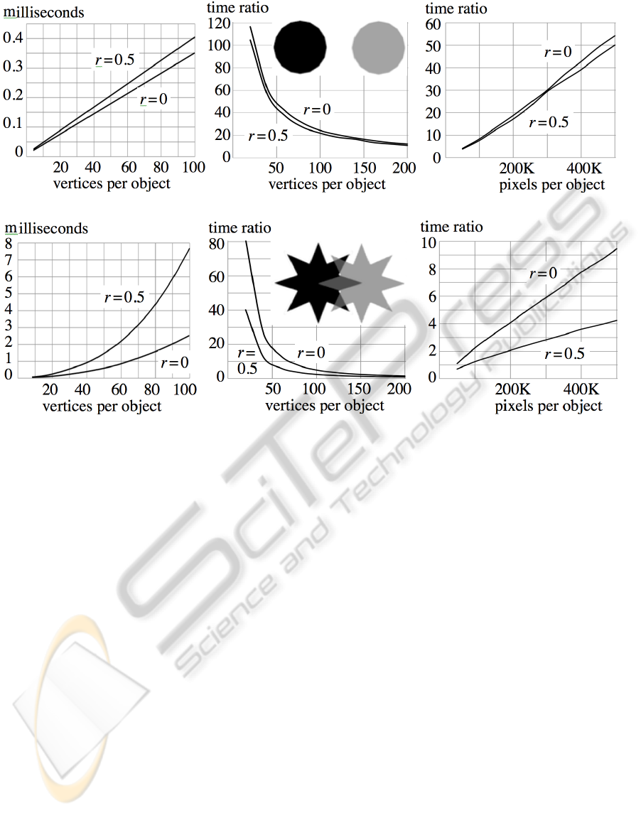
θ+π/2. Figures 5 and 6 show examples of objects

and related force histograms, and Fig. 7 shows the

processing times of crisp objects in a best case

scenario (a)(b)(c) and in a worst case scenario

(d)(e)(f). Note, (a)(d), that the processing time is

minimum when r = 0, maximum when r is not an

integer (all non-integer r values give about the

same processing times), and between these two

extremes when r is a nonzero integer. Times to

process objects in vector vs. raster forms are

compared in (b)(c)(e)(f). For example, (e),

calculating the histogram of constant forces (r = 0)

between two intersecting stars with 50 vertices each

(i.e., 25-pointed stars) is about 20 times faster if the

stars are in vector form (than if they are in raster

form and made of 250K pixels each; whatever the

raster algorithm used). Note that for every r and

every pair of objects considered in these

experiments, the histograms produced by the vector

and raster algorithms are visually indistinguishable,

and their similarity (as measured by the Tanimoto

index) is greater than 99.6%.

5 CONCLUSIONS

A relative position descriptor like the histogram of

forces which is endowed with remarkable properties

and able to handle any pair of 2-D objects (whether

these objects are crisp or fuzzy, connected or

disconnected, with or without holes, disjoint or

overlapping) is undoubtedly a most useful tool:

relative position descriptors are a natural complement

to colour, texture, and shape descriptors; the spatial

organization of 2-D objects is a subject of interest in

many disciplines; spatial regions are modelled by

fuzzy sets in an increasing number of applications

and areas; examples of regions with holes or

multiple connected components abound; examples

of regions that touch or overlap abound as well (in

particular,

fuzzy regions

often

naturally

overlap).

(a) (b) (c) (d)

Figure 5: (a) Britain and Ireland share Northern Ireland. (b) Bolivia in South America. (c) Canada and the U.S. (d) The risk

for strong or violent tornadoes in the U.S. is high (black), medium (dark gray), low (light gray), negligible (elsewhere).

(a) (b) (c) (d) (e) (f)

Figure 6: Examples of force histograms. In (a), the objects are disjoint (Canada relative to South America). In (b), they

touch (Canada relative to the U.S.). In (c), they overlap (Britain relative to Ireland). In (d), they are equal (the U.S.). In (e),

one includes the other (South America and Bolivia). In (f), one is crisp (the U.S.) and the other is fuzzy (tornado risk map).

ICPRAM 2012 - International Conference on Pattern Recognition Applications and Methods

(a) (b) (c)

(d) (e) (f)

Figure 7: Processing times; in each case, forces were computed in 100 evenly distributed directions. In (a)(b)(c), the objects

are crisp disjoint regular convex polygons; in (d)(e)(f), they are crisp intersecting star polygons. In (a)(d), the objects are in

vector form and the processing time is the average processing time per direction; note that in (a), only the directions with

nonzero forces were actually considered. In (b)(c)(e)(f), the time ratio is the time to process the two objects in raster form

divided by the time to process the same two objects in vector form. In (b)(e), each raster object is made of 250K pixels; in

(c)(f), each vector object has 100 vertices.

Until now, however, only objects in raster form

could be considered. In this paper, we have widened

the scope of the histogram of forces to objects in

vector form. Since polygons are a fundamental type

of data in, e.g., computer graphics and GIS, and are

also often used to approximate boundaries of raster

regions, this is a significant achievement which

should draw the interest of practitioners. Note that all

the programs for force histogram computation are

freely available upon request. We are currently

developing efficient general algorithms for the

handling of 3-D raster and vector objects.

ACKNOWLEDGEMENTS

The authors want to express their gratitude for

support from the Natural Science and Engineering

Research Council of Canada (NSERC), grant

262117.

REFERENCES

Matsakis, P., Wendling, L., 1999. A New Way to Repre-

sent the Relative Position of Areal Objects. In IEEE

Trans. on Pattern Analysis and Machine Intelligence,

21(7), 634-643.

Matsakis, P., Wendling, L., Ni, J., 2011. A General

Approach to the Fuzzy Modeling of Spatial Rela-

tionships. In Jeansoulin, R., Papini, O., Prade, H.,

Schockaert, S. (Eds.): Methods for Handling Imperfect

Spatial Information, Springer-Verlag, 49-74.

Ni, J., Matsakis, P., 2010. An Equivalent Definition of the

Histogram of Forces: Theoretical and Algorithmic Im-

plications. In Pattern Recognition, 43(4), 1607-1617.

Shyu, C. R., Klaric, M., Scott, G. J., Barb, A. S., Davis, C.

H., Palaniappan, K., 2007. GeoIRIS: Geospatial In-

formation Retrieval and Indexing System—Content

Mining, Semantics Modeling, and Complex Queries.

In IEEE Trans. on Geoscience and Remote Sensing,

45(4), 839-852.

Sjahputera, O., Keller, J. M., 2007. Scene Matching Using

F-Histogram-Based Features with Possibilistic C-

A GENERAL ALGORITHM FOR CALCULATING FORCE HISTOGRAMS USING VECTOR DATA

Means Optimization. In Fuzzy Sets and Systems,

158(3), 253-269.

Skubic, M., Perzanowski, D., Blisard, S., Schultz, A.,

Adams, W., Bugajska, M., Brock, D., 2004. Spatial

Language for Human-Robot Dialogs. In IEEE Trans.

on Systems, Man, and Cybernetics Part C, 34(2),

154-167.

Vaduva, C., Faur, D., Gavat, I., 2010. Data Mining and

Spatial Reasoning for Satellite Image Characterization.

In Proceedings of the 8

Int. Conf. on Communica-

tions (COMM), 173-176.

Wang, Y., Makedon, F., Drysdale, R. L., 2004. Fast

Algorithms to Compute the Force Histogram. Pattern

Recognition.

ICPRAM 2012 - International Conference on Pattern Recognition Applications and Methods