PUTATIVE MATCH ANALYSIS

A Repeatable Alternative to RANSAC for Matching of Aerial Images

Anders Hast

1,2

and Andrea Marchetti

The Centre for Image Analysis, Uppsala University, Lägerhyddsvägen 2, Uppsala, Sweden

Institute of Informatics and Telematics, Consiglio Nazionale delle Ricerche, Via G. Moruzzi 1, Pisa, Italy

Keywords: RANSAC, Feature Matching, Image Stitching, Aerial Photos.

Abstract: One disadvantage with RANSAC is that it is based on randomness and will therefore often yield a different

set of inliers in each run, especially if the dataset contains a large number of outliers. A repeatable algorithm

for finding both matches and the homography is proposed that will yield the same set of matches every time

and is therefore a useful tool when trying to evaluate other algorithms involved and their parameters.

1 INTRODUCTION

In the process of finding corresponding points in two

or more images it necessary to determine which

points are true matches, so called inliers, and which

points are not matching, so called outliers. RANSAC

(Fishler and Bolles, 1981) is one of the far most used

algorithms for this purpose and many variants have

been proposed in literature (Chum et al., 2003;

Chum et al., 2004; Chum and Matas, 2005. Chum

and Matas, 2008; Michaelsen et al., 2006. Sattler et

al., 2009). The main disadvantage with RANSAC is

that it is not repeatable (Zuliani, 2009) since it is

based on random sampling, as the name itself

suggests: RANdom SAmple Consensus. Hence it is

difficult using RANSAC while trying to run tests of

other algorithms involved and changing their

parameters, as the set of inliers may vary in each

run.

We propose a repeatable algorithm that is not

based on randomness, which will find the same

inliers and thus the same homography (Vincent and

Laganiere, 2001) every time the same set of matches

is given to the algorithm. As it performs an analysis

based on the putative matches, we have chosen to

call it Putative Match Analysis or PUMA for short.

2 PUTATIVE MATCH ANALYSIS

The first step of PUMA is to construct what we have

chosen to call a Relative Polar Matrix (RPM). The

matrix is constructed in the following way as shown

in figure 1.

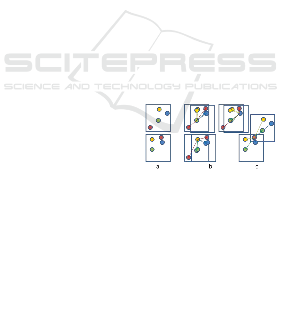
Figure 1: The RPM is constructed by taking the matches in

the two images (a) and translating all matches one at a

time so that one point coincide (b). A pair of vectors are

constructed from that point to each pair of inliers. When a

true match is used as base it will yield vectors with close

to equal relative length and angle for true matches but not

for false ones. A false match (c) on the other hand will

yield varying cosines and lengths.

The two matched images (a) are translated so

that one matching pair coincide, one at a time and

each of these comparisons are shown in the four

images to the right (b, c). First of all the green match

is translated so the points overlap and the relative

length of the vector from this point to a matching

pair as well as the cosine of the angle between these

are computed for all putative matches. The relative

length of these vectors 



and 



is:

 =

min

(











)

max

(











)

(1)

341

Hast A. and Marchetti A..

PUTATIVE MATCH ANALYSIS - A Repeatable Alternative to RANSAC for Matching of Aerial Images.

DOI: 10.5220/0003802603410344

In Proceedings of the International Conference on Computer Vision Theory and Applications (VISAPP-2012), pages 341-344

ISBN: 978-989-8565-04-4

 2012 SCITEPRESS (Science and Technology Publications, Lda.)

Hence both the cosine of the angle:  between

vectors and relative length: r will always be in the

interval

[

1. .1

]

and

[

0. .1

]

respectively. The first

column of the matrix will contain the results for this

first match and each row contains the pairs of

(

, 

)

to each pair of matches. Those that are true inliers

(the yellow and blue), will yield similar values of

(

, 

)

even if the images have different rotation and

scale. However, the false matches will yield pairs of

(

, 

)

that have different values. Similarly when a

false match coincide (c), all putative matches will

yield quite different values of

(

, 

)

. This procedure

is repeated for each match, hence the second column

will contain the pairs relative to this match and so

on.

The first example of using this algorithm is

shown in figure 2 where one of the images is rotated

and scaled down just to show that the technique

works well for both cases.

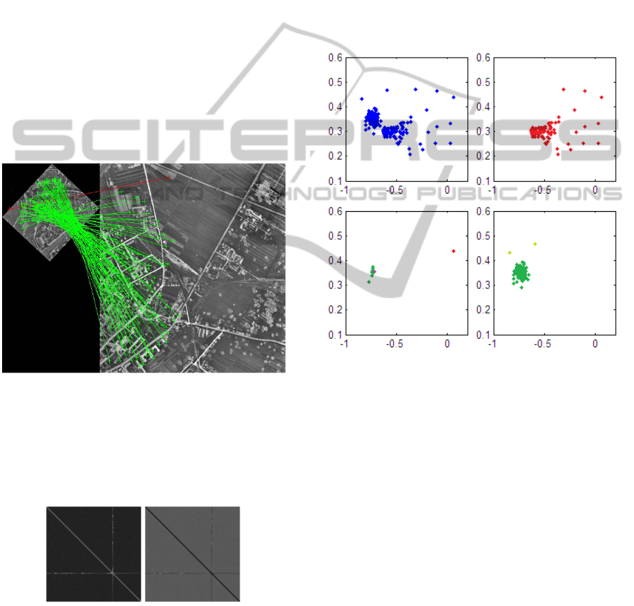
Figure 2: Matching of two aerial images where one of

them is rotated and scaled. The method proposed finds the

outlier in red even for this extreme situation.

In figure 3 the RPM matrix is visualized showing

one matrix for , to the right and one for , to the

left.

Figure 3: The RPM matrix is visualized showing one

symmetric matrix for , to the left and one for  in the

middle. In this case there is just one outlier giving a clear

trace in the matrices.

Each one of them are symmetric so all the

information could be packed into one matrix as the

diagonal contains no information as the points

cannot be compared to themselves. In this example

there is one outlier that gives a clear trace in the

matrix as its value differs from the others that are

similar.

The second step of PUMA can be performed in

several ways using the clustering technique of your

choice. Each column in the RPM matrix contains a

cluster that can be visualized using

(

, 

)

as co-

ordinates. Figure 4 upper left shows all points in the

RPM plotted in the same plot and obviously it is

hard to say what cluster we are looking for.

Figure 4: The upper left: all points in the RPM. Upper

right: one set of the RPM is used in the plot and clearly it

contains an outlier as it is quite scattered. Bottom left: a

set containing an inliers is used and the outlier (red) is

seen far from the cluster center (violet). Bottom right: the

outlier has been removed and the whole RPMS is plotted

and the cluster contains only putative inliers.

In the upper right the set that corresponds to the

outlier is plotted. As expected the points are more

scattered. In the bottom left one set is plotted and the

outlier, depicted in red, is clearly seen far from the

centre, depicted in violet. In the bottom row right the

whole RPM is plotted after removing the outlier so

that it now contains putative inliers. Still there are a

couple of points lying a bit off centre that can be

dealt with by choosing a smaller threshold for the

clustering.

Clustering can be done in many ways (Jain and

Dubes) and k-means clustering (MacQueen, 1967)

is one popular clustering algorithm. Nevertheless,

the problem here is a bit different as there is one

cluster set for each row (or column as the RPM is

VISAPP 2012 - International Conference on Computer Vision Theory and Applications

342

symmetric after removing any doubles) and the

columns are also related to each other. PUMA was

developed to work for aerial images, which will

form one cluster that we search for. The clustering

approach used here is very simple and starts by

computing the average 



for each row  of

(

, 

)

thus giving a “centre” that is a bit perturbed by the

outliers. Then the distance between each point on the

row

(





, 



)

and 



is stored in a matrix, which we

have chosen to call the Relative Distance Matrix

(RDM). In each iteration the set with an outlier

furthest away from the average centre is located and

that outlier is therefore removed and the RDM is

updated accordingly.

In figure 4 bottom left is in fact the set having

the largest distance shown. The outlier is easily

found by locating the column with the largest value.

In this case it is column 65 that has its largest value

in row 9, indicating that it is the set with number 65

(column and row) that must be deleted as it gave the

largest distance for set number 9. So even if it is set

number 65 that is shown in the upper right in the

picture, it is actually set number 9 in the lower right

that helps us finding the most extreme outlier.

3 RESULTS

Two areal images, shown in figure 5, with different

orientation were used and in order to produce more

false matches the Harris operator (Harris and

Stephens 1988) was used instead of the more

accurate SIFT (Lowe, 2004). In this case the there

were about 84.4% of false matches.

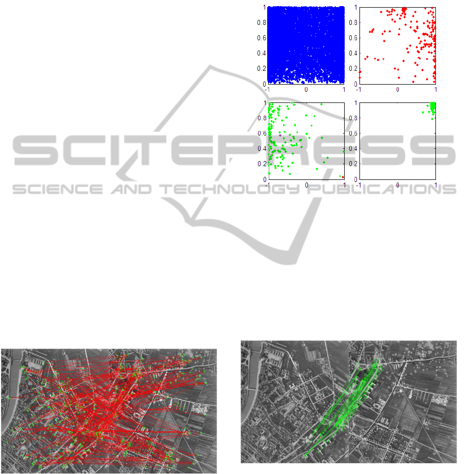
Figure 5: Putative matches produced using the Harris

detector, with about 84.4% false matches.

In figure 6 is shown the whole set of clusters

plotted in the top left and the set corresponding to

the most extreme outlier in the top right where the

cluster is obviously scattered. In the bottom left

there is the set with the largest distance between the

centre and a point, ie. an outlier and will be removed

later in the algorithm. In the bottom right is the

result after removing all outliers down to a certain

threshold.

Figure 6: The upper left: all points in the RPM. Upper

right: one outliers set of the RPM, which clearly contains

an outlier as it is quite scattered. Bottom left: a set

containing another outlier (red) and the cluster centre

(violet) has the maximum distance. Bottom right: all the

outliers have been removed and the whole RPM is plotted

and the cluster contains only putative inliers.

The cluster is found in the upper right corner,

which corresponds to a little scaling and a small

rotation, about 18 degrees. The result contains all 34

columns regarded as inliers by the algorithm.

Figure 7: The result after executing the PUMA algorithm.

Out of 218 putative matches 34 were chosen as inliers.

Figure 7 shows the result of PUMA yielding 34

inliers out of 218 putative matches. It should be

noted that the basic implementation of RANSAC did

not come to a correct consensus due to the high

amount of outliers, however by forcing RANSAC to

PUTATIVE MATCH ANALYSIS - A Repeatable Alternative to RANSAC for Matching of Aerial Images

343

continue it found all inliers after an average of about

32000 iterations.

Figure 8 shows both the RPM and the RDM for

the whole set as well as for the case when 5 outliers

are remaining. Clearly it is hard to see which rows

and columns to remove in the upper row, while it

becomes more and more clear as the outliers are

removed.

Figure 8: The RPM matrix is visualized showing one

symmetric matrix for , to the left and one for  in the

middle. And the RDM to the right. In the upper row is the

whole set and in the lower row (scaled to be larger) is the

set with five remaining outliers that gives a clear trace in

the matrices.

The homography can be computed using this set

of inliers and the set of inliers can easily be pruned

using ordinary RANSAC by setting a desired

threshold. As all matches are regarded as inliers

RANSAC will now without problem find all inliers

within that specific threshold.

4 CONCLUSIONS

The PUtative Match Analysis (PUMA) is a

repeatable, brute force algorithm that can be used

whenever it is necessary to test other parameters in

an application and when it is crucial that the set of

inliers are always the same for the same set of data.

Hence, it can be used as a robust tool for testing and

development of computer vision applications with

small non affine distortions as in the aerial images

used as examples. Due to its high computational cost

it will be outperformed by RANSAC in most

situations, but when there are many outliers, PUMA

can be a good choice for a reasonable number of

matches as it has proven to find the inliers even for a

rather high amount of noise in the set.

ACKNOWLEDGEMENTS

This work was carried out during the tenure of an ERCIM

"Alain Bensoussan" Fellowship Programme at IIT,

CNR in Pisa, Italy.

REFERENCES

Capoyleas, V., Rote, G. and Woeginger, G., 1991.

Geometric Clusterings, J. Algorithms, vol. 12, pp. 341-

356.

Chum, O., Matas, J., Kittler, J., 2003. Locally Optimized

RANSAC. In DAGM-Symposium. 236-243.

Chum, O., Matas, J and Obdrzalek, S., 2004. Enhancing

RANSAC by generalized model optimization. In

Proceedings of the Asian Conference on Computer

Vision (ACCV).

Chum, O. and Matas, J., 2005. Matching with PROSAC -

Progressive Sample Consensus. In Proceedings of the

IEEE Computer Society Conference on Computer

Vision and Pattern Recognition (CVPR). pp 220-226.

Chum, O. and Matas, J., 2008. Optimal randomized

ransac. IEEE Transactions on Pattern Analysis and

Machine Intelligence, 30(8). pp1472–1482.

Fischler, M. A. and Bolles, R. C., 1981. Random sample

consensus: A paradigm for model fitting with

applications to image analysis and automated

cartography, Communications of the ACM, 24, pp.

381–395.

Harris, C., Stephens, C., 1988. A Combined corner and

edge detection. In Proc. of The Fourth Alvey Vision

Conference, pp. 147–151.

Jain, A. K. and Dubes, R. C., 1988. Algorithms for

Clustering Data. Englewood Cliffs, N.J.: Prentice

Hall.

Lowe, D. G., 2004. Distinctive Image Features from

Scale-Invariant Keypoints, International Journal of

Computer Vision, 60, 2, pp. 91-110.

MacQueen, J. B., 1967. Some Methods for classification

and Analysis of Multivariate Observations,

Proceedings of 5-th Berkeley Symposium on

Mathematical Statistics and Probability, Berkeley,

University of California Press, vol 1, pp. 281-297.

Michaelsen, E., von Hansen, W., Kirchhof, M., Meidow,

J., Stilla, U., 2006. Estimating the Essential Matrix:

GOODSAC versus RANSAC, PCV06, pp.1-6.

Sattler, T., Leibe, B., Kobbelt, L., 2009. SCRAMSAC:

Improving RANSAC's efficiency with a spatial

consistency filter. ICCV 2009: pp. 2090-2097.

Vincent, E. and Laganiere, R., 2001. Detecting planar

homographies in an image pair. Image and Signal

Processing and Analysis, pp. 182–187.

Zuliani, M., 2009. RANSAC for dummies. pp. 42.

http://vision.ece.ucsb.edu/~zuliani/Research/RANSAC

/docs/RANSAC4Dummies.pdf

VISAPP 2012 - International Conference on Computer Vision Theory and Applications

344