A LAYOUT ALGORITHM FOR THE VISUALIZATION

OF MULTIPLE RELATIONS IN GRAPHS

G´eraldine Bous

SAP Research Sophia Antipolis, Business Intelligence Practice, Av. Dr. Maurice Donat 805, 06250 Mougins, France

Keywords:

Visualization Algorithms, Hierarchical Graph Drawing, Multiple Relations, Structural Constraints.

Abstract:

Many recent applications involve data models that rely on heterogeneous graphs (multiple node and relation

types). Drawing these graphs is more difﬁcult than drawing standard graphs, as it is desirable to take into

account the heterogeneity of graphs in the form of constraints, possibly stemming from user preferences,

to compute the layout. In this paper we propose a method for hierarchical graph drawing that is based on

structural constraint modeling. These constraints are combined with crossing minimization algorithms to yield

the desired visual effect. Three types of constraints are considered and illustrated, giving special attention to

the drawing of multiple relations for interactive graph visualization.

1 INTRODUCTION

Graph Drawing serves the purpose of determining a

layout, i.e. a representation in the plane, such that a

graph can be visualized and analyzed by a user. This

involves, for example, making all components of a

graph visible (vertices, edges, attribute values, labels,

etc.), addressing crossings, etc. Although the disci-

pline has a long and solid history (see, e.g., (Battista

et al., 1999) for an overview), several recent appli-

cations have opened new research challenges in the

area. A key example is the drawing of the hetero-

geneous graphs that arise in the modeling of systems,

networks and knowledgestructures - models that need

a proper visual representation in order to be under-

stood and analyzed by users.

In this paper, we address the problem of hetero-

geneous graph drawing on the basis of (user) con-

straints. We present a method that captures the het-

erogeneity of a graph by incorporating several types

of ‘visual constraints’ directly into the graph. By vi-

sual constraints, we refer to requirements on the ﬁnal

layout of graph. For example, the user may specify

constraints relative to the order of certain nodes, wish

to visualize nodes clustered by type or simply require

the simultaneous visualizations of multiple relations

(i.e. multiple graphs) on a unique set of nodes. We

focus on hierarchical graph drawing (Sugiyama et al.,

1981) and model the constraints structurally, i.e. not

using parametric approaches, but rather by incorpo-

rating the constraints into the graph itself.

The paper is structured as follows: we describe the

problem and give a brief overview of related work in

section 2. The adaptation of hierarchical graph draw-

ing algorithms to incorporate structural constraints is

discussed in section 3. Next, we address the drawing

of graphs with multiple relations (section 4) and pur-

sue with extensions of our approach to other types of

visual constraints (section 5). We ﬁnally conclude in

section 6.

2 PROBLEM DESCRIPTION &

RELATED WORK

Traditionally, graph drawing algorithms are centered

towards the drawing of homogeneous graphs, i.e.

graphs in which all nodes and edges are alike. In other

words, it is in general assumed that graphs are com-

posed of abstract entities, i.e. vertices, that all are of

the same type; similarly, the edges of the graph are

simply assumed to be abstract connections (between

the vertices) that share the same properties. Modern

information and knowledge models are however fre-

quently built on the basis of heterogeneous graphs.

For example, semantic models involve different types

of nodes and relations. Likewise, business oriented

social networks can be designed to contain more than

just connections between employees: it is possible

to incorporate the hierarchical structure of the com-

pany, extra-hierarchical structures that model cross-

690

Bous G..

A LAYOUT ALGORITHM FOR THE VISUALIZATION OF MULTIPLE RELATIONS IN GRAPHS.

DOI: 10.5220/0003865106900700

In Proceedings of the International Conference on Computer Graphics Theory and Applications (IVAPP-2012), pages 690-700

ISBN: 978-989-8565-02-0

 2012 SCITEPRESS (Science and Technology Publications, Lda.)

organizational projects and teams, as well as other

types of entities and relations like furniture (e.g., cars

with relationships like ‘drives’ or ‘maintains’), data

transfer processes, budgets, etc. These last examples

are actually only a few of the actual user requests we

have encountered in practice in the context of soft-

ware design for business social networks. The reader

may refer to (Cuvelier et al., 2012) for more details.

2.1 Challenges in Drawing

Multi-relational Graphs

The main challenge in visualizing multiple relation-

ships, or, to be more general, in visualizing several

graphs deﬁned on a common set of vertices, is not the

visualization of the graphs themselves. It is indeed

possible to visualize the different graphs separately

using state-of-the-art graph drawing algorithms (Bat-

tista et al., 1999; Herman et al., 2000, are excellent

surveys). However, a visualization approach based

on ‘multiple views’, each showing one relation at a

time, makes it difﬁcult to show the ‘true’ connectivity

in the network and is hence impractical for analysis

purposes. Hence, the challenge resides in deciding

how multiple relations should be displayed, possibly

simultaneously and/or offering the possibility for user

interaction.

First, it must be decided whether all relationships

should be visualized at the same time or whether it is

better to approach the problem in an interactive man-

ner, allowing the user to select a subset of relation-

ships. We advocate the use of the second solution:

indeed, not all users may want to visualize the same

relationships, which calls for an interactive approach

where the user selects what she wants to see. Also,

the simultaneous representation of all relationships

may lead to visually loaded graphs that are visually

intractable and inappropriate for analysis.

The choice of an interactive approach to the vi-

sualization of multiple relationships may, in turn, be

approached in several ways. The simplest solution to

this problem actually consists in selecting a reference

graph, e.g. a hierarchical structure, and to superpose

the other graphs on demand. This approach requires

the computation of the optimal layout for the hierar-

chical structure and, as the user selects or un-selects

other relationships, the layout is updated by adding

new edges (resp. removing them) without changing

the position of the nodes. The main criticism of such

an approach is that it is likely to lead to a large num-

ber of edge crossings, which are usually considered to

be undesirable for the understanding and analysis of

the graph.

A second solution would be to re-compute a new

layout every time the user selects (or de-selects) a re-

lationship. As long as the number of nodes is rea-

sonable, it is indeed possible to optimize the layout

for a speciﬁc subset of graphs in real-time. Although

this approach would produce a much more appeal-

ing visual output, there is one important disadvantage:

adding as little as one relation to a given (current) dis-

play may lead to a complete disruption of both node

and edge locations. Indeed, what is optimal, e.g. in

terms of edge crossings, for a given set of relation-

ships, is not granted to be optimal for another one.

Re-optimization is thus problematic in that it destroys

the mental map of the user (Misue et al., 1995), which

requires her to re-adapt to the new display. Intuitively,

but also experimentally, it has been shown that this is

not desirable (Purchase, 2000; Purchase et al., 2006;

Saffrey and Purchase, 2008).

The question is thus whether it is possible to com-

pute a layout that would simultaneously be optimal

in the sense of edge-crossings and preserve the men-

tal map of the user as she navigates from one sub-

set of relationships to another. The two criteria may

nonetheless be antagonistic, as minimizing the num-

ber of crossings is totally independent from – and a

priori unrelated to – the idea of preserving the men-

tal map (i.e. the vertex positions in two-dimensional

space).

In this paper, we propose an approach designed to

meet both criteria. The general idea is to pre-compute

an optimal layout, in terms of crossings, for an ag-

gregated graph containing all relationships. As the

user selects (resp. un-selects) relationships, edges and

nodes are just added (resp. removed), but their loca-

tions do not need to change (as the layout is optimal

for all relationships).

2.2 Related Work

As the reader will see shortly, the work presented here

is essentially that of visualizing several graphs on the

same set of nodes at the same time. From this per-

spective, the topic is related to the drawing of com-

pound graphs. A compound graph is a graph com-

posed of a directed tree and one adjacency graph.

The few contributions to the resolution of this prob-

lem generally focus on sub-cases where the adjacency

graph only connects nodes not having common ances-

tors (Sugiyama and Misue, 1991; Bertault and Miller,

1999; Forster,2002) and represent the inclusion nodes

as rectangular containers. The work of (Raitner,

2004) is an extension to (Sugiyama and Misue, 1991)

that addresses the immersive visualization of the tree

structure. The work discussed in (Holten, 2006) uses

a technique based on edge-bundling and illustrates the

A LAYOUT ALGORITHM FOR THE VISUALIZATION OF MULTIPLE RELATIONS IN GRAPHS

691

use of other container representations than rectangles

(hierarchical drawings, treemaps, etc.). Our work dis-

tinguishes itself from the research topics mentioned

above in two ways. First, in the topic it addresses: the

modeling of ‘visual constraints’ for the visualization

of graphs containing heterogeneous data. Second, in

the algorithmic approach used here, which is based on

structural constraints in combination with a hierarchi-

cal graph drawing algorithm.

The work of (Shen et al., 2006) addresses the vi-

sualization of social network graphs, where, like is

the case in this paper, several relationships may exist

between nodes. (Shen et al., 2006) use the descrip-

tion of these relationships, called ‘ontology’, to ﬁl-

ter and cluster the original graph data into meaningful

agglomerates; in contrast, our work addresses the vi-

sualization of the relationships themselves, ideally in

such a way that the result is visually tractable. (Fekete

et al., 2003) use a treemap-basedapproach to visualiz-

ing a hierarchy and set of additional edges or relation-

ships, the latter being drawn ‘on top’ of the treemap.

The problem addressed is thus similar, but the goal of

the method is different: our approach seeks to orga-

nize the layout in such a way that requirements on it

(i.e. the visual constraints) can be met.

In the forthcoming section, we review the algo-

rithmic procedure for drawing hierarchical graphs.

We explain how a generic structural constraint is mod-

eled and embedded into a graph and at what stage this

occurs in the algorithmic process.

3 HIERARCHICAL GRAPH

DRAWING WITH

STRUCTURAL CONSTRAINTS

In this section we describe a methodology to adapt

traditional hierarchical graph drawing algorithms to

the case of graphs that are to be drawn taking ac-

count visual constraints in view of computing a lay-

out that enables the interactive visualization of mul-

tiple relations. The only requirement on the visual

constraints is that they have to be modeled as graphs.

More speciﬁcally, the approach we discuss here con-

sists in aggregating the constraints and the hierarchi-

cal structure into a single graph that can be drawn

with state-of-the-art algorithms. The key element to

turning the structural constraints into the desired vi-

sual constraints is achieved thanks to ‘design’ of the

structural constraints in combination with the cross-

ing minimization step. In this section, we describe

the approach in its general form; speciﬁc types of con-

straints are addressed in sections 4 and 5.

3.1 Problem Formulation and Notations

Let H(V, E) be a hierarchy, i.e. a directed acyclic tree

of vertices v ∈ V and edges (v, w) ∈ E with E ⊆ V ×V.

In parallel, let there be I (directed or undirected)

graphs G

, E

), i ∈ I, with V

∩ V 6=

0 (i.e. V

not restricted to V

⊂ V, but both must have a least

one node in common). The heuristic method we dis-

cuss here is based on four distinct steps. First, the

layering step that determines the layer y(v) at which

every node v ∈ H of the tree should be placed. Sec-

ond, an aggregation phase to embed H and the con-

straints G

into a unique directed tree H

with ver-

tices V

and edges E

(note that V ⊆ V

). The third

step determines the order o(v) of the vertices in ev-

ery layer of H

with the purpose of minimizing the

number of edge crossings. The ﬁnal step reﬁnes the

horizontal position x(v) of every vertex for the screen

layout. The reader should note that the steps one,

two and four correspond to the steps of the Sugiyama

algorithm (Sugiyama et al., 1981). It is also worth

emphasizing that, although we here focus on trees,

the Sugiyama algorithm – and hence the method pre-

sented here – can be extended to graphs in general; the

reader may refer to (Battista et al., 1999) for details.

3.2 Layering

The ﬁrst step of our approach computes the vertical

position y(v) of the vertices of the hierarchy v ∈ H.

It is important to note that the layer computed at this

level is maintained throughout the different steps of

the algorithm: the layer of a node v ∈ V hence is iden-

tical in the trees H and H

Several methods can be used to assign a layer to

the nodes of a directed tree (Battista et al., 1999); we

use the shortest path method, that is, a method that as-

signs every node to the layer immediately below that

of its closest predecessor. Let

(i, j) =



1 if (i, j) ∈ E

0 otherwise.

(1)

If δ

(i, j) = 1, it means that the vertices i and j are

connected by an edge directed towards j. Solving the

following linear program provides the vertical coordi-

nates of the nodes of the hierarchy H (note that layer

1, the top layer, is assigned to the root of the tree):

min

∑

i∈V

y(i)

s.t. y( j) − y(i) ≥ 1 if δ

(i, j) = 1

y(i) ≥ 1 ∀i ∈ V.

(2)

IVAPP 2012 - International Conference on Information Visualization Theory and Applications

692

3.3 Graph Aggregation

The graph aggregation step concerns the embedding

of the structural constraints into the hierarchy H. In

general terms, the aggregation step consists in per-

forming the union of the graphs, i.e.

= H

[

i=1

, (3)

where H

denotes the aggregated graph. The satisfac-

tion of the visual constraints is attained by the embed-

ding in combination with the crossing minimization

step discussed below. More precisely, the constraints

must be designed in such a way that they lead to cross-

ings in H

when they are not satisﬁed. The detailed

modeling of different types of constraints and the cor-

responding aggregation procedures are discussed in

sections 4 and 5.

3.4 Crossing Minimization

The crossing minimization problem of hierarchical

graphs is generally approached by minimizing the

crossings of all pairs of consecutive layers in the tree.

This problem, known as the “two-layer crossing prob-

lem”, is NP-hard, which justiﬁes the existence of sev-

eral heuristic methods to solve it. In the context of

constrained graph drawing, we seek to minimize not

only the crossings in the hierarchy H, but also the

crossings that would arise through the violation of the

structural constraints. In other words, crossings are

minimized for the set of vertices {v ∈ V

| y(v) = k}

and {v ∈ V

| y(v) = k+ 1} for k = 1, ..., y

max

)−1,

where y

max

denotes a function that returns the maxi-

mum depth of a tree. The goal of the two-layer cross-

ing problem is to determine the order in which the

vertices of the two layers should be placed as to min-

imize the number of crossings between the edges that

connect them. Two well known and well documented

techniques are the “median heuristic” and the “swap

heuristic”, that exist in several variants and generally

demand the use of dummy (temporary) vertices to

lead to good results. The interested reader may refer

to (Battista et al., 1999) and the references therein for

a detailed description of these two, as well as other,

heuristic methods.

3.5 Final Coordinate Assignment

Once the horizontal order of the vertices of H

has

been determined, two distinct steps must actually be

performed. First, all dummy vertices introduced in

previous steps must be removed. This includes those

added to model structural constraints, as well as those

added during the crossing minimization step. The ﬁ-

nal step consists in reﬁning the horizontal coordinates

of the remaining vertices (i.e. those of H), without

changing their order, to obtain a more uniform and vi-

sually attractive result on the screen. Several methods

exist to this purpose, some of which are documented

in (Battista et al., 1999).

4 AGGREGATION FOR

MULTI-RELATIONAL GRAPHS

In this section we describe the application of graph

drawing with structural constraints to the case of

multi-relational graphs, which we illustrate by the

joint visualization of linear processes, in view of al-

lowing an interactive visualization without disrupting

the mental map of the user. The different relations are

embedded into the hierarchical graph in order to com-

pute a layout that is optimal, in terms of crossings, for

any subset of relations the user may want to explore.

We ﬁrst discuss the modeling of the constraints as

graphs, as well as the aggregation process (which was

presented in a generic manner in section 3.3); next we

provide some experimental results regarding the com-

putational complexity of our approach.

4.1 Approach Description

Like previously, let H(V, E) be a hierarchy and

, E

) be a series of I graphs, i ∈ I, with V

⊆ V.

We consider the special case where every G

mod-

els a linear process, that is, a sequence of vertices

, v

, ..., v

), where n

represents the length of pro-

cess i. Each process is thus a separate graph - a rela-

tion - on different, not necessarily disjoint, subsets of

The method of structural constraints makes it pos-

sible to model proximity and adjacency constraints

for nodes in H. This type of constraints cannot be

taken into account in traditional hierarchical graph

drawing and are necessary to visualize the process in

both in a ‘linear way’ and to restrict each process to

a well deﬁned portion of the (visual representation of

the) hierarchy. The constraints are designed to force

the vicinity of vertices that are connected to each

other and have been assigned the same layer in the

y-coordinate determination step (section 3.2); in addi-

tion, this minimizes the number of edges that cross the

layout from one side to another. For example, in the

illustration of ﬁgure 1(a), superposing the linear pro-

cess on the hierarchy implies both edge crossings and

same-layer traversing edges (from vertex B to vertex

E).

A LAYOUT ALGORITHM FOR THE VISUALIZATION OF MULTIPLE RELATIONS IN GRAPHS

693

The aggregated graph H

is built in I steps: start-

ing with the hierarchy alone, each graph G

is inte-

grated sequentially. The constraints are modeled ac-

cording to the pseudocode below:

for k = 1 to n

if y(v

i,k

) 6= y(v

i,k+1

) then

if y(v

i,k

) < y(v

i,k+1

) then

i,k

, v

i,k+1

) = 1

else

i,k+1

, v

i,k

) = 1

end if

else

add temporary vertex v

to H

y(v

) = y(v

i,k

) + 1

i,k

, v

) = 1

i,k+1

, v

) = 1

end if

end for

If two consecutive vertices in process G

are not in

the same layer, they are connected in H

with an edge

directed from the lower layer vertex to the higher level

vertex (root-to-leaf direction), in order to avoid creat-

ing cycles. To the contrary, if two consecutivevertices

in G

have the same layer, a constraint is added in or-

der to enforce a placement in which the two vertices

will be direct neighbors. This constraint is modeled

on the basis of a temporary vertex v

that is connected

to and placed below the two process vertices. Figure

1(b) illustrates this principle.

The application of the crossing minimization pro-

cedure on the aggregated graph H

achieves the vi-

sual consistency for the joint visualization of the hi-

erarchy and the linear processes. Indeed, the connec-

tion of process vertices thanks to temporary vertices

and edges in the ‘aggregated hierarchy’ H

forces the

proximity of process vertices. Intuitively, it is clear

that, the further away two process vertices are from

each other (i.e. the more other vertices are placed be-

tween them), the greater the number of edge crossings

will be. The principle is illustrated in ﬁgures 1(b) and

1(c), that, respectively, show the aggregated hierarchy

before and after crossing minimization. The ﬁnal re-

sult of this method, i.e. after removal of temporary

vertices, is shown in ﬁgure 1(d).

When several relations exist on the same hierar-

chy, pre-computing the layout for all relations simul-

taneously with this technique allows determining a vi-

sual representation that is optimal for the aggregated

graph, i.e. for all relations. It is hence easy to use

an interactive approach where to user is allowed to

select the relations that she wants to visualize by sim-

ply adding or hiding the corresponding edges without

modifying the layer and order of the vertices, thereby

maintaining the her mental map.

4.2 Experimental Results

The main drawbacks of hierarchical graph drawing

algorithms are the computation time and, if heuris-

tic methods are used to compensate for the computa-

tional complexity, the potential sub-optimality of the

solutions also becomes a disadvantage. The computa-

tional complexity of our method is higher than that of

drawing the base hierarchy alone, as the aggregated

graph H

contains a certain number of dummy ver-

tices to model the structural constraints. It is thus of

interest to determine the impact of the number of pro-

cess nodes (and indirectly of the number of process

dummy vertices) on the average computation time

with the algorithm proposed in the previous section.

We have performed an experimental evaluation of

the crossing minimization step of the algorithm, i.e.

the step with highest computational complexity. The

algorithm implements the median heuristic in Matlab.

We evaluated the computation time for randomly gen-

erated trees of size n and one or more linear processes.

More precisely, for every randomly generated tree, a

total of lp nodes, where lp is a random number satis-

fying 2 ≤ lp ≤ n, were assigned to one or more linear

processes (we thus have lp =

∑

). We measure the

average computation time for every pair (n, lp). Note

that the actual number of nodes is larger than n, not

only due to the structural constraint approach, but also

due to the other dummy vertices that are needed in the

algorithm (crossing minimization step).

We performed a total of 55700 tests with 5 ≤ n ≤

230 and 5 ≤ lp ≤ min(n, x

max

· y

max

), where x

max

and

max

are, respectively, the maximum width and depth

of a tree. The scatter plot in ﬁgure 2(a) shows the

CPU time (in seconds) as a function of the number of

nodes n in the base tree. The color code used for the

dots is a function of lp. More precisely, lp has been

divided into six equal parts, with each color assigned

to an interval: blue < cyan < green < yellow < ma-

genta < red. The scatter plot in ﬁgure 2(b) shows the

CPU time (in seconds) as a function of the number of

process nodes lp. Again, we divide the outcomes in

six categories, this time according to the size of the

tree n, and use the same color code as above. The

purpose of the color code is to show if there is a cor-

relation between the CPU time and the variable that

is not shown. That is, for ﬁgure 2(a) the color code

shows the impact of lp on a plot that shows (n, f(n));

for 2(b), the color gives a hint of the impact of n on a

plot that shows (lp, f(lp)).

An analysis of both ﬁgures leads to the follow-

ing conclusion: the decisive factor in the computation

time is n, the size of the base tree. Indeed, when show-

ing (n, f(n)), we can see that lp has but little correla-

IVAPP 2012 - International Conference on Information Visualization Theory and Applications

694

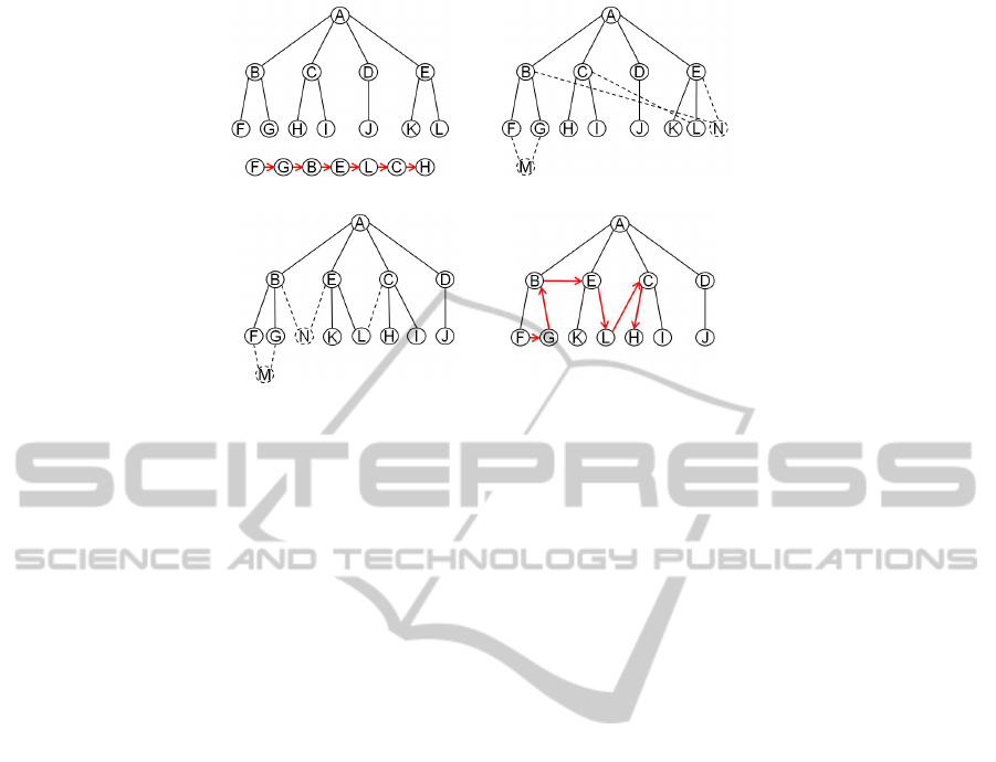
(a) Hierarchy and process. (b) Structural constraints.

Figure 1: Example of a structural constraint to embed a linear process into a tree. The edge-crossing minimization step in

combination with the structural constraint allows visualizing the process in a linear manner, without traversing edges.

tion since the ‘color code’ is randomly distributed in

the cloud of data-points (note that a correlation is vis-

ible for lower values of n as lp ≤ n). This is con-

ﬁrmed by the scatter plot (lp, f (lp)), which shows an

almost perfectly horizontal cloud with layered colors.

Hence, higher CPU time is correlated essentially to

n and not to lp – which implies that the method of

structural constraints does not have a signiﬁcant neg-

ative impact on the computational complexity and on

the performance of the algorithm.

In addition to the problem of computational com-

plexity, we have tested the quality of the method here

proposed with respect to the number of crossings.

Both the hierarchies and linear processes used for the

tests are randomly generated and approximately 5000

tests were run. The reference for the comparison is

a tree whose layout is determined by the ‘standard

Sugiyama algorithm’ (with the Swap Heuristic), but

where no processing is done on the nodes of the lin-

ear processes. In other words, the edges of the lin-

ear processes are simply drawn ‘on top’ of the tree.

The average number of crossings was then determined

both as a function of n and lp. Figure 3(a) shows the

ratio of the average number of crossings without pro-

cessing to the average number of crossings with our

method as function of n; similarly ﬁgure 3(b) shows

the ratio as a function of lp. The ﬁrst ﬁgure shows

that the structural constraints method is particularly

efﬁcient for n < 50, where no processing doubles the

number of crossings. In general, it appears that our

method improves the result by approximately 25%.

As for the second ﬁgure, as function of lp, the trend

is more steady, with a 20% improvement in favor of

our method.

5 EXTENSION TO OTHER TYPES

OF CONSTRAINTS

The technique of structural constraints described in

section 3 can be easily extended to other types re-

quirements than those of representing multiple rela-

tions (linear processes) in a visually consistent man-

ner. In this section we illustrate how to perform the

graph aggregation for two additional types of con-

straints on hierarchical graphs: ﬁrst, the clustered vi-

sualization of multiple node types and, second, for or-

der constraints on a subset of the nodes of the hierar-

chy.

5.1 Visual Node Clustering in

Hierarchical Graphs

For graph-based data structures – here assumed hier-

archical – that contain different node types (e.g. per-

sons, furniture, etc.), it may be desirable to draw the

graph such that nodes of the same type are shown to-

gether, thereby forming clusters of identical nodes.

Like for multi-relational graphs, this can be achieved

by designing adequate structural constraints that are

embedded into the tree structure, previous to the

crossing minimization step.

As usual, let H(V, E) denote the hierarchy; more-

over, assume that every node in the hierarchy has

a given type i, where i = 1, ..., I. In this case, we

deﬁne the structural constraints as graphs G

, E

such that V

= {v

∪ (v ∈ V | type(v) = i)} and E

{(v

, v) | v ∈ V

\ v

}. In other terms, we deﬁne a con-

straint graph for every node type; the graph is com-

A LAYOUT ALGORITHM FOR THE VISUALIZATION OF MULTIPLE RELATIONS IN GRAPHS

695

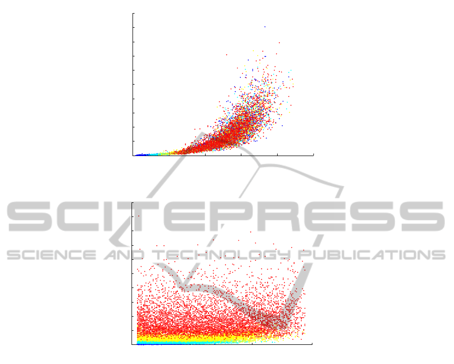
0 50 100 150 200 250

0.5

1.5

2.5

3.5

4.5

no. of nodes

CPU time (s)

(a) CPU as a function of n.

0 50 100 150

0.5

1.5

2.5

3.5

4.5

no. of process nodes

CPU time (s)

(b) CPU as a function of lp.

Figure 2: Computational complexity of our method. The ﬁgures show that higher CPU time is correlated essentially to n and

not to lp.

posed of a temporary vertex v

that is connected to all

nodes of H that have type i.

The constraint graphs are built and embedded se-

quentially into the hierarchy H, forming the aggre-

gated hierarchy H

. Initializing H

as H, the process

for the aggregation of one graph G

is described be-

low:

add temporary vertex v

to H

y(v

) = y

max

(H) + 1

for all v ∈ V | type(v) = i do

(v, v

) = 1

end for

The temporary vertex, symbolizing the cluster for

a given node type, is added on the ﬂy as the constraint

is embedded into the hierarchy. Temporary vertices

are placed one layer below all nodes of H, i.e. at layer

max

(H) + 1 (so that y

max

) = y

max

(H) + 1), and

connected to all vertices of type i.

The ‘clustering effect’ is again obtained thanks to

the combined use of structural constraints and a cross-

ing minimization algorithm on the graph H

. Indeed,

mixing nodes of different types creates crossings on

the (temporary) edges that bind the nodes to their cor-

responding ‘cluster vertex’; the constraints and the

crossing minimization thus implicitly induce horizon-

tal regions that, whenever possible, contain nodes of

one speciﬁc type. This is illustrated in ﬁgure 4, where

we use the same base hierarchy as in ﬁgure 1 with

nodes in three colors to symbolize their types (ﬁg-

ure 4(a)). Figures 4(b) and 4(c) respectively show

the aggregated hierarchy graph before and after the

crossing minimization; the ﬁnal result, after removal

of dummy vertices and edges, is shown in ﬁgure 4(d).

IVAPP 2012 - International Conference on Information Visualization Theory and Applications

696

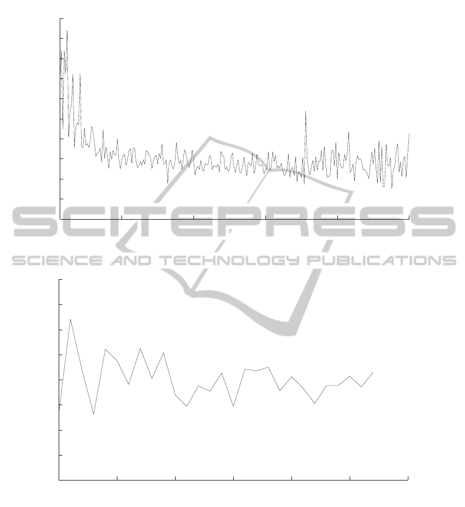
50 100 150 200 250

0.5

0.75

1.25

1.5

1.75

2.25

2.5

2.75

no. of nodes

ratio of average no. of crossings

(a) Crossing ration as function of n.

5 10 15 20 25 30 35

1.05

1.1

1.15

1.2

1.25

1.3

1.35

1.4

no. of process nodes

ratio of average no. of crossings

(b) Crossing ration as function of lp.

Figure 3: Ratio of the average number of crossings without processing to the average number of crossings with the structural

constraints technique.

5.2 Vertex Order Constraints

The use of structural constraints also enables the end-

user to specify order constraints on a subset of the

vertices of the tree H. Again, the idea is to design the

constraints in such a way that the application of the

crossing minimization algorithm on the aggregated

graph H

forces the satisfaction of the constraints.

Let, as usual, H(V, E) denote the hierarchy and

assume that there exists a subset of vertices V

⊆ V

for which the (relative) order is deﬁned, i.e. o(v

) <

o(v

) < ... < o(v

) for v

∈ V

. If the aggregated

A LAYOUT ALGORITHM FOR THE VISUALIZATION OF MULTIPLE RELATIONS IN GRAPHS

697

(a) Hierarchy and types. (b) Structural constraints.

Figure 4: Example of a structural constraint to cluster the nodes of a tree according to their type.

hierarchy is initialized as H

= H, then an order con-

straint can be embedded into the hierarchy with the

following procedure:

for i = 1 to |V

| with v

∈ V

add temporary vertex v

to H

y(v

) = y

max

(H) + 1

o(v

) = i

, v

) = 1

if i > 1 then

i−1

, v

) = 1

end if

end for

The process described therein is quite simple: for

each ordered node v

, one dummy vertex is added be-

low the hierarchy (i.e. y(v

) = y

max

(H) + 1) and is

connected to v

. Since the order of the dummy vertex

is imposed (o(v

) = i) it sufﬁces to apply the cross-

ing minimization excluding the dummy vertex layer,

i.e. taking the edges into account but without reorder-

ing the nodes, to impose an order on the vertices of

∈ V

. Without the if-loop and the constraint added

at line 7, the order of the nodes will be preserved by

the crossing minimization algorithm, but may only be

a relative order. That is, no constraints restrict other

nodes (v ∈ V \V

) to be placed in between the nodes

of V

. If the end-user prefers a strict order, then it is

necessary to add an additional constraint that connects

a vertex v

∈ V

not only to its corresponding dummy

vertex v

, but also to that of its successor in the order

relation.

An illustration for this case would be quite simi-

lar to the one we used for the linear process in ﬁgure

1; indeed, a linear process, as deﬁned in section 4,

is nothing but a strict linear order (see, e.g., (Roman,

2008) for an exhaustive deﬁnition of order relations).

In the case of order constraints, the modeling is how-

ever different: all temporary vertices are placed in the

bottom layer so that the crossing minimization algo-

rithm can be applied only to the layers of the original

tree H.

To conclude this section, we emphasize that the

use of structural constraints is not limited to the con-

straints we discuss here. For example, it is con-

ceivable to combine ordering constraints with cluster-

ing constraints or constraints relative to multiple rela-

tions.

6 DISCUSSION AND FUTURE

WORK

We have introduced the concept of structural con-

straints and shown how these can be used to model

visual constraints for heterogeneous graphs. The con-

straints are designed as to be treated by crossing min-

imization algorithms. We explored three different

cases, with their respective constraints, to which the

method can be applied. We give particular focus to

the visualization of multiple relations, showing how

our technique can be used for the computation of lay-

outs destined to interactive graph visualization with-

out having a signiﬁcant impact on the base compu-

tational complexity of algorithm, dominated by the

crossing minimization step.

While it is certainly conceivable to design speciﬁc

algorithms for each of the examples given here, the

advantage of using structural constraints is precisely

to offer the possibility to embed the constraints di-

rectly into the data. Consequently, it is possible to

use generic state-of-the-art hierarchical graph draw-

ing algorithms without further modiﬁcations. From

IVAPP 2012 - International Conference on Information Visualization Theory and Applications

698

the perspective of large scale software design, the use

of generic, reusable and extensible modules are crite-

ria of capital importance, which our method allows to

satisfy.

Although the method presented here produces

good results, further experiments are required to val-

idate it for larger graphs, as well as to analyze its

applicability when different types of constraints are

combined together. The quality of the results is

highly impacted by the quality of the output provided

by the heuristic methods used in the crossing mini-

mization step. This imposes further research on us-

ing this method in combination with other types of

approaches and visualization techniques, like those

presented in (Burch and Diehl, 2008; Burch et al.,

2010) for the visualization of time-varying compound

graphs. Interesting is also the work of (Shen et al.,

2006), as well as the approach presented in (Muelder

and Ma, 2008), which combines clustering techniques

and tree-maps for fast layout computation of large

graphs. Another important direction for future re-

search is related to the non-discriminative applica-

tion of crossing algorithms. The embedding of all

relations and constraints into a unique graph makes

it impossible to discriminate edge and node types

(constraint, hierarchy, relation, etc.). When no zero-

crossing solutions exist, it is impossible for current

crossing minimization algorithms to distinguish be-

tween ‘favorable’ and ‘unwanted’ crossings. For

example, the end-user may specify that she prefers

crossings in the hierarchy rather than in the linear pro-

cesses she visualizes. Hence, the design of algorithms

that can prioritize crossings according to the edge and

node types is an important next step to consider.

Heterogeneous graph drawing, in general, is a

topic rich in challenges where many problems remain

to be addressed. These range from the user experi-

ence domain (e.g. adequate layout criteria and ‘coher-

ent’ visual representations), the management of zoom

in/out approaches following several criteria, to the in-

teractivity with respect to the visible subset of rela-

tions themselves.

ACKNOWLEDGEMENTS

The work presented here was developed in the context

of the ARSA project (Analyse des R´eseaux Sociaux

pour Administrations), partially funded by the French

DGCIS (Direction G´en´erale de la Comp´etitivit´e, de

l’Industrie et des Services). The author wishes to

thank our end-user, the City Administration of An-

tibes, with a special mention to our contact, Patrick

Duverger.

REFERENCES

Battista, G. D., Eades, P., Tamassia, R., and Tollis, I. G.

(1999). Graph Drawing: Algorithms for the Visual-

ization of Graphs. Prentice Hall, Upper Saddle River.

Bertault, F. and Miller, M. (1999). An algorithm for draw-

ing compound graphs. In Proceedings of the 7th In-

ternational Symposium on Graph Drawing (GD’99),

pages 197–204.

Burch, M. and Diehl, S. (2008). Timeradartrees: Visualiz-

ing dynamic compound digraphs. In Proceedings Eu-

rographics/ IEEE-VGTC Symposium on Visualization

2008, volume 27, pages 823–830.

Burch, M., Fritz, M., Beck, F., and Diehl, S. (2010). Time-

spidertrees: A novel visual metaphor for dynamic

compound graphs. In Hundhausen, C. D., Pietriga, E.,

Daz, P., and Rosson, M. B., editors, Proceedings of the

IEEE Symposium on Visual Languages and Human-

Centric Computing VL/HCC 2010, pages 168–175.

Cuvelier, E., Bous, G., Aufaure, M.-A., and Kleser, G.

(2012). ARSA: Analyse des R´eseaux Sociaux pour

les Administrations - une exp´erience d’int´egration de

r´eseaux sociaux internes et externes dans une admin-

istration. Ing´enierie des Syst`emes d’Information. To

appear.

Fekete, J.-D., Wang, D., Dang, N., and Plaisant, C. (2003).

Overlaying graph links on treemaps. In IEEE Sympo-

sium on Information Visualization Conference Com-

pendium (demonstration).

Forster, M. (2002). Applying crossing reduction strate-

gies to layered compound graphs. In Proceedings of

the 10th International Symposium on Graph Drawing

(GD’02), pages 276–284.

Herman, I., Melanon, G., and Marshall, S. (2000). Graph

visualization and navigation in information visualiza-

tion: A survey. IEEE Transactions on Visualization

and Computer Graphics, 6:24–43.

Holten, D. (2006). Hierarchical edge bundles: Visualiza-

tion of adjacency relations in hierarchical data. IEEE

Transactions on Visualization and Computer Graph-

ics, 12:741–748.

Misue, K., Eades, P., Lai, W., and Sugiyama, K. (1995).

Layout adjustments and the mental map. Journal of

Visual Languages and Computing, 6:183–210.

Muelder, C. and Ma, K.-L. (2008). A treemap based method

for rapid layout of large graphs. In Proceedings of

Visualization Symposium, 2008. PaciﬁcVIS ’08. IEEE

Paciﬁc, pages 231 –238.

Purchase, H. (2000). Effective information visualization:

a study of graph drawing aesthetics and algorithms.

Interacting with Computers, 13:147–162.

Purchase, H., Hoggan, E., and Grg, C. (2006). How impor-

tant is the “mental map”? an empirical investigation

of a dynamic graph layout algorithm. In Proceedings

of 14th International Symposium on Graph Drawing

(GD’06), pages 184–195.

Raitner, M. (2004). Visual navigation of compound graphs.

In Proceedings of the 12th International Symposium

on Graph Drawing (GD’04), pages 403–413.

A LAYOUT ALGORITHM FOR THE VISUALIZATION OF MULTIPLE RELATIONS IN GRAPHS

699

Roman, S. (2008). Lattices and Ordered Sets. Springer,

New York.

Saffrey, P. and Purchase, H. (2008). The “mental map” ver-

sus “static aesthetic” compromise in dynamic graphs:

a user study. In Proceedings of the 9th Conference on

Australasian User Interface, pages 85–93.

Shen, Z., Ma, K.-L., and Eliassi-Rad, T. (2006). Visual

analysis of large heterogeneous social networks by se-

mantic and structural abstraction. IEEE Transactions

on Visualization and Computer Graphics, 12:1427 –

1439.

Sugiyama, K. and Misue, K. (1991). Visualization of struc-

tural information: Automatic drawing of compound

digraphs. IEEE Transactions on Systems, Man, and

Cybernetics, 21:876–892.

Sugiyama, K., Tagawa, S., and Toda, M. (1981). Methods

for visual understanding of hierarchical system struc-

tures. IEEE Transactions on Systems, Man, and Cy-

bernetics, 11:109–125.

IVAPP 2012 - International Conference on Information Visualization Theory and Applications

700