Trajectory Tracking Control by LMI-based Approach for Car-like
Robots
Nicoleta Minoiu Enache
Renault SAS, Technocenter, 1 Avenue de Golf, 78288 Guyancourt, France
Keywords:
Trajectory Tracking, Car-like Vehicle, Passenger Vehicle, LMI Optimization.
Abstract:
A lot of research has been done concerning motion planning and trajectory tracking control for robots, includ-
ing car-like robots. Nevertheless, most of the methods require very well defined trajectories, continuous and
several times derivable. Frequently, the system has to be written in a specific form, like the chained form, and
the path obtained in the original space may not satisfy additional constraints in the original space or singulari-
ties can occur in the control law. The goal of this work is to investigate a control method to do the trajectory
tracking control of car-like robots in the original space, which does not require trajectories several times deriv-
able, but with good robustness and pursuit properties in order to implement it on a passenger vehicle. The
control law for trajectory tracking presented here is derived from a method developed for unicycles. This is
based on a real time combination of static linear feedbacks that are obtained by an off line LMI (Linear Matrix
Inequalities) approach.
1 INTRODUCTION
Under the assumption of no slippage, the car-like
robots are non-holonomic vehicles, which are global
controllable but not without challenging control prob-
lems due to their inherent constraints on the trajectory.
For asymptotic stabilization of fixed configurations
the Brockett’s theorem proves for car-like robots the
non-existence of pure-state feedbacks (Brockett et al.,
1983). The research in control theory has then looked
for more complex methods than the pure-static feed-
backs, mainly classified in two fields: the fixed point
stabilization, for instance for the parking maneuvers,
and the tracking of feasible trajectories. The topic of
the present paper is included in this last field, more
specifically the trajectory tracking for passenger ve-
hicles at low speeds is addressed.
A trajectory is considered feasible if it comes from
a reference car-like vehicle. In real-time applications,
under constraints coming from obstacles for instance,
most of the reference trajectories are not entirely fea-
sible, even if they are sufficiently smooth. However,
the non-feasibility does not imply the impossibility to
follow a such trajectory with non-zero small bounded
errors. This is called practical stabilization by (Morin
and Samson, 2009).
In the literature two types of trajectories are de-
scribed for the control of car-like robots. The analytic
trajectories are smooth, several times derivable and
can take into account the vehicle motion constraints
(Montes et al., 2007), (Levinson et al., 2011). On the
opposite, the trajectories can be expressed as vectors
of points linked by segments which are only based on
environnement constraints (Leedy et al., 2006).
Depending on the trajectory type, feedback con-
trol laws have been developed to do the trajectory
tracking. For smooth, several times derivable tra-
jectories, the control problem has been solved el-
egantly, either by flatness approach (Brault et al.,
2000) or by transposing the vehicle kinematic model
into the chained-form. Once transposed into the
chained form, several control techniques can be em-
ployed, like for instance the exact feedback lineariza-
tion (DeLuca et al., 1998) or the backstepping (Mnif,
2004). Although relying on solid proofs for stabil-
ity, the chained form control approaches present the
weakness of the locality of the chained form transfor-
mation and the difficulty to guarantee control proper-
ties for the original space.
If the trajectory is given only by a set of points,
most of the time expressed in the vehicle frame, con-
trol approaches like the pure-pursuit, geometric Stan-
ley method (Snider, 2009) or Nonlinear Model Pre-
dictive Control (NMPC) (Zhu, 2008) have been ap-
plied. Stability proofs are difficult to provide for
all the three mentioned control techniques. More-
38
Minoiu Enache N..
Trajectory Tracking Control by LMI-based Approach for Car-like Robots.
DOI: 10.5220/0004017300380047
In Proceedings of the 9th International Conference on Informatics in Control, Automation and Robotics (ICINCO-2012), pages 38-47
ISBN: 978-989-8565-22-8
Copyright
c
 2012 SCITEPRESS (Science and Technology Publications, Lda.)

over, while the pure-pursuit method and the geomet-
ric Stanley method are extremely easy to implement
in real time (Snider, 2009), the NMPC is much more
difficult since it requires complex online optimization
(Falcone et al., 2007). At higher speeds, a lineariza-
tion of the dynamic vehicle model has been carried
out and more advantageous real time algorithms for
MPC have been used by (Levinson et al., 2011). The
pursuit performances for the pure-pursuit method and
the geometric Stanley method depend on the calibra-
tions, especially the look-ahead distance. For trajec-
tories with very low radius, like the turn-around ma-
neuvers, the calibration of the look-ahead distance is
challenging (Campbell, 2007).
Simpler wheeled mobile robots than the car-like
vehicles are the unicycles. The control laws dedicated
to unicycles have been developed separately from the
car-like robots due mainly to the difference in the con-
trol inputs: yaw rate and longitudinal velocity for the
unicycle and steering angle and longitudinal veloc-
ity for the car-like robot. Some examples for control
laws for unicycle robots are given in (Kim and Tsio-
tras, 2002). Not all control laws developed for uni-
cycle robots can be used directly for car-like robots.
A rotation of the car-like robot is the result of a first
order dynamic driven by the steering angle, hence
delayed with respect to the unicycle. However, re-
cently (Michałek and Kozłowski, 2011) have shown
that control techniques developed for the unicycles
can be implemented also for the car-like robots with
very good results under some conditions.
The control approaches by convex optimization,
and implicitly by LMI methods, have had an impor-
tant spread out in the last twenty years with the devel-
opment of the theoretical methods (Boyd et al., 1994),
(Scherer and Weiland, 2004), (Chilali and Gahinet,
1996), followed by the evolution of the computa-
tion algorithms and toolboxes (Mattingley and Boyd,
2010), (Grant and Boyd, 2011), (L¨ofberg, 2004).
For the control of the motion of passenger cars,
these methods have been especially used for the driv-
ing assistance systems at higher speeds. Advanta-
geously, the dynamic vehicle model can be linearized
considering a constant longitudinal speed, hence the
LMI methods can be employed. Afterwards, the de-
signed control law has to be tested on its robustness
against speed variations. The lateral vehicle control
has been investigated by (Li et al., 2005), (Minoiu
et al., 2009), the longitudinal control makes the object
of the works (Mammar and Yacine, 2012), (Enache
et al., 2009) and the yaw rate control is treated in (Mi-
noiu et al., 2010).
For lower speeds, in particular in the range where
the kinematic vehicle model is still valid, the control
approachby LMI optimization has not been employed
yet for the car-like robots to the author’s knowledge.
On the robotic field, the LMI approach has been im-
plemented for the trajectory tracking control of uni-
cycles in (Gonzalez et al., 2009), (Gonzalez et al.,
2010) in order to tackle problems related to the slip-
page of the unicycle wheels and to obtain robustness
for a large area of possible reference trajectories.
The work presented here investigates an LMI ap-
proach for control design addressed to an autonomous
car-like (passengers) vehicle at low speed, for exam-
ples less than 20km/h. The primary goal is to obtain
a robust control for this range of speeds, expressed
in the original vehicle space and which can be eas-
ily implemented in real time under constraints related
to a passenger vehicle. To this end, the method used
for the unicycles in (Gonzalez et al., 2009) is adapted
for the car-like vehicle application. This method is
completed with further necessary constraints in or-
der to satisfy assumptions described in (Michałek and
Kozłowski, 2011). These assumptions ensure feasi-
bility and good quality for the car-like vehicle control.
The next section 2 presents the kinematics of the
unicycle and of the car-like robot and the necessary
conditions to use control laws originally developed
for unicycles to control car-like robots. In section 3
the control law for the unicycle robot is casted as an
LMI convex optimization problem under constraints.
Subsequently, the obtained control law is translated to
the car-likerobot inputs. Simulation results are shown
in section 4 for two vehicle models: one is a kinematic
car-like vehicle model and a second is a complex pas-
senger vehicle model. Conclusions in section 5 wrap
up the paper.
2 VEHICLE MODEL AND ERROR
DYNAMICS
The range of speeds addressed in this paper for the
autonomous passenger vehicle makes difficult the
choice of a vehicle model. At very low speeds, below
5km/h, the kinematic vehicle model can be success-
fully used to control its trajectory (Rajamani, 2006).
When the speed increases, the tires start to deform es-
pecially for high lateral or longitudinal accelerations
and the assumption of no slippage is no longer valid.
A dynamic vehicle model is then necessary to take
this into account. On the other side, the tire mod-
els, like for instance Pacejka model, are not precise
at low speed, usually lower than 20km/h. This lets
a gap between 5km/h and 20km/h where any of the
well known vehicle models is not especially recom-
mended. The choice done in this study is to work
TrajectoryTrackingControlbyLMI-basedApproachforCar-likeRobots
39

with the car-like kinematic model which is valid for
low speeds and to test the robustness of the designed
control law also at higher speeds and accelerations.
This will be later seen in the simulations done with
the model of a real passenger vehicle in section 4.
2.1 Car-like Robot and Unicycle
Kinematics
In order to apply to the car-like robot feedback con-
trollers originally designed for unicycle robots, the
car-like kinematics have to be written in a new form,
as the equations of a unicycle kinematics and the
remaining steering dynamics as in (Michałek and
Kozłowski, 2011).
The car-like robot kinematics have the following
equations







˙x = vcosθ
˙y = vsinθ
˙
θ =
v
L
tanδ
˙
δ = u
(1)
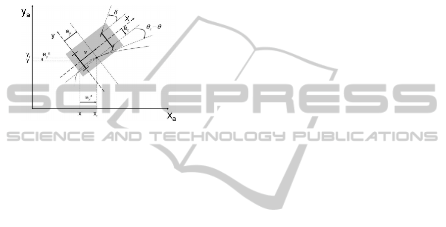
where (x, y, θ) is the pose of the middle point of the
rear axle of the car-likerobot in an absolute frame, v is
the velocity considered at the middle point of the rear
axle and δ is the steering angle of the front wheels (see
Figure 1). Defining a new input ω =
v
L
tanδ, equation
(1) can be rewritten as:



˙x = vcosθ
˙y = vsinθ
˙
θ = ω
(2)
˙
δ
= u
(3)
If a control law is designed for the unicycle robot
described by (2) with the control inputs (v,ω)
T
, the
desired velocity v
car
and the desired steering angle
δ
car
have to be recovered in order to control the car-
like robot. The transformation is given by:
v
car
= v
δ
car
= sat(atan(
Lω
v
),δ
max
)
(4)
where δ
max
is the maximum steering angle of the front
wheels. It can be noticed that this transformation has
a singularity for the case v = 0. The occurrence of this
case is discussed largely in (Michałek and Kozłowski,
2011). In this application a numerical parade is used
to avoid this situation by setting δ
r
= 0 and
˙
δ
r
= 0 for
v < ε, ε very small.
As visible in equation (3), the steering dynamics
can not be imposed instantaneously, hence a steering
angle stabilizer controller is necessary. This steering
angle stabilizer can have the expression
u = K
d
sgn(e
δ
)|e
δ
|
α
+
˙
δ
car
(5)
as described in (Michałek and Kozłowski, 2011),
where e
δ
= δ
car
− δ, K
d
> 0 and α ∈ (0, 1].
A reference trajectory is represented in Figure 1
by a dotted line and is described by (x
r
, y
r
, θ
r
) in the
absolute frame. It is assumed that this trajectory has
been created by an unicycle, which kinematics are:



˙x
r
= v
r
cosθ
r
˙y
r
= v
r
sinθ
r
˙
θ
r
= ω
r
(6)
where v
r
is the longitudinal speed and ω
r
the yaw rate
of the reference unicycle robot.
The posture error is defined by e
a
=
(e
a
x
, e
a
y
, e
a
θ
)
T
= (x
r
− x, y
r
− y, θ
r
− θ)
T
in the
absolute frame and by e = (e
x
, e
y
, e
θ
)
T
in the frame
related to the car-like robot as shown in Figure
1. In the following it is supposed that there exist
control laws (v,ω) that stabilize asymptotically
the kinematics of the unicycle robot in equation
(2) to the reference trajectory (x
r
, y
r
, θ
r
) and that
these control laws depend on the posture error
(u,ω)
T
= (u(e
a
),ω(e
a
))
T
.
If the following conditions on the reference trajec-
tory (x
r
, y
r
, θ
r
) and on the control laws (v,ω) are sat-
isfied, (Michałek and Kozłowski, 2011) have shown
that δ converges to δ
car
following equations (3) and
(5) and that the car-like robot trajectory [x, y, θ]
T
converges asymptotically to the reference trajectory
[x
r
, y
r
, θ
r
]
T
(Michałek and Kozłowski, 2011):
1. (x
r
, y
r
, θ
r
)
T
satisfies equation (6) and is continu-
ously and derivable several times.
2. |
˙
θ
r
˙x
r
cos(θ
r
)+ ˙y
r
sin(θ
r
)
| ≤ |
tan(δ
max
)
L
|
3.
∂(v,ω)
T
∂(e
a
x
,e
a
y
,e
a
θ
)
T
∈ L
3
∞
,
∂(v,ω)
T
∂t
∈ L
2
∞
4. |
ω
v
| ≤ |
1
L
tan(δ
max
)| for almost all t > 0
Condition (1) means that control laws using time
derivatives of the reference trajectory can be imple-
mented and that the reference trajectory is feasible for
the unicycle robot model (2). Hence the asymptotic
convergence can be obtained. Condition (2) imposes
a limited curvature to the reference trajectory that is
achievable with the maximum steering angle of the
car-like robot δ
max
, if δ
max
<
π
2
. Condition (3) en-
sures boundedness of the time derivatives of the con-
trol inputs, necessary for the stabilizing control law
(5) when the derivative
˙
δ
car
is computed from equa-
tion (4). Finally, condition (4) reflects the feasibility
of the control laws designated for the unicycle robot
by the car-like robot. This condition on the control
law completes condition (2) which is related to the
reference trajectory. Condition (4) can be violated for
time instants without impeding the asymptotic behav-
ior.
ICINCO2012-9thInternationalConferenceonInformaticsinControl,AutomationandRobotics
40

2.2 Error Dynamics of the Unicycle
Kinematics
The relation between e
a
and e is described by the well
known relation (Oelen and van Amerongen, 1994):
e =


cosθ sinθ 0
−sinθ cosθ 0
0 0 1


e
a
= Te
a
(7)
Figure 1: Car-like robot in a global frame (Oelen and van
Amerongen, 1994).
The next step is to compute the dynamics of the
errors of the unicycle part of the car-like robot with
respect to the reference trajectory in the car-like robot
coordinates frame. The derivative of the error in ab-
solute frame yields from equations (2) and (6)



˙e
a
x
= v
r
cosθ
r
− vcosθ
˙e
a
y
= v
r
sinθ
r
− vsinθ
˙e
a
θ
= ω
r
− ω
(8)
After derivation of equation (7) and introduction of
equation (8), the dynamics of the errors of the unicy-
cle part of the car-like robot are obtained as:



˙e
x
= v
r
cose
θ
+ ωe
y
− v
˙e
y
= v
r
sine
θ
− ωe
x
˙e
θ
= ω
r
− ω
(9)
Since these relations are not linear, a linear Taylor
approximation with limited number of terms around
zero can be employed. It yields a time variant error
model:


˙e
x
˙e
y
˙e
θ


=


0 ω
r
0
−ω
r
0 ω
r
0 0 0




e
x
e
y
e
θ


+
+


1 0
0 0
0 1



v
r
− v
ω
r
− ω

(10)
Written in a more compact form this model has
the following expression:
˙e = A(t)e+ Bz, z = (v
r
− v,ω
r
− ω)
T
(11)
A(t) =


0 ω
r
0
−ω
r
0 v
r
0 0 0


B =


1 0
0 0
0 1


(12)
Even if the state matrix A varies in time, an important
property is obtained since its elements are the refer-
ence yaw rate and the longitudinal speed which are
bounded:
v
r
∈ [v
min
r
; v
max
r
]
ω
r
∈ [ω
min
r
; ω
max
r
]
(13)
Indeed, the matrix A varies inside a convex enve-
lope with the vertices defined by the yaw rate and the
longitudinal speed bounds:
A(t) ∈ A = Co{A
1
, A
2
, A
3
, A
4
}
A
1
= A(v
min
r
,ω
min
r
), A
2
= A(v
min
r
,ω
max
r
),
A
3
= A(v
max
r
,ω
min
r
), A
4
= A(v
max
r
,ω
max
r
)
(14)
3 TRAJECTORY TRACKING
CONTROLLER BY LMI
APPROACH
First, a control law is deduced for the unicycle robot.
In a second step, this control law is translated to feed
the car-like robot inputs.
The implemented control law is a linear feedback
z = Ke issued from a linear combination of static lin-
ear feedbacks. These are valid for each vertex of the
convex set (13) as implemented in (Gonzalez et al.,
2009) for unicycles with wheels slippage. The LMI
approach is advantageous since it allows to show sta-
bility and satisfaction of constraints for the whole
variation range of v
r
and ω
r
. The linear feedbacks
are denoted by:
K
i
∈ R
2×4
, i = 1,... 4, (15)
one for each couple
R = {(v
min
r
,ω
min
r
), (v
min
r
,ω
max
r
), (v
max
r
,ω
min
r
), (v
max
r
,ω
max
r
)}
(16)
At each time instant, (v
r
,ω
r
) satisfying (13) and the
matrix A(t) can be written as
(v
r
,ω
r
) =
∑
4
i=1
λ
i
R (i)
A(t) =
∑
4
i=1
λ
i
A
i
∑
4
i=1
λ
i
= 1, λ
i
≥ 0, i = 1,.. . ,4
(17)
If the gain K is defined by
K =
4
∑
i=1
λ
i
K
i
(18)
TrajectoryTrackingControlbyLMI-basedApproachforCar-likeRobots
41

and z = Ke, then the closed loop system has the ex-
pression:
˙e =
4
∑
i=1
λ
i
A
i
e+
4
∑
i=1
λ
i
BK
i
e =
4
∑
i=1
λ
i
(A
i
+ BK
i
)e (19)
3.1 Stability and Poles Placement
The stability at each vertex of A is ensured for the
closed loop system with the feedbacks z = K
i
e, if
there exist P ≻ 0, P = P
T
such that the Lyapunov
LMIs hold (Boyd et al., 1994):
(A
i
+ BK
i
)
T
P+ P(A
i
+ BK
i
) ≺ 0, i = 1,...,4 (20)
The sum of the above inequalities, after multiplication
with λ
i
, keeps the property of negative definite, and
hence the stability for the closed loop system (19) is
achieved. By multiplying the above inequalities (20)
with Q = P
−1
at the right and at the left and by denot-
ing Y
i
= K
i
Q, it yields linear matrix inequalities:
QA
T
i
+ A
i
Q+Y
T
i
B
T
+ BY
i
≺ 0, i = 1, ...,4 (21)
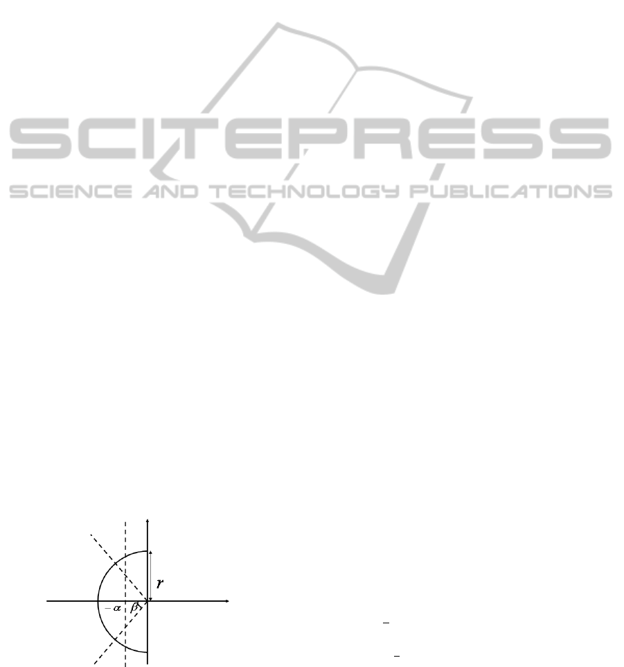
In (Chilali and Gahinet, 1996) further LMI con-
straints are deduced to complete the stability condi-
tion with pole placement constraints:
QA
T
i
+ A
i
Q+Y
T
i
B
T
+ BY
i
+ 2αQ ≺ 0 (22)

−rQ A
i
Q+ BY
i
QA
T
i
+Y
T
i
B
T
−rQ

≺ 0 (23)

M
i
sinβ N
i
cosβ
N
i
cosβ M
i
sinβ

≺ 0, (24)
where M
i
= QA
T
i
+A
i
Q+Y
T
i
B
T
+BY
i
and N
i
= A
i
Q−
QA
T
i
+ BY
i
− Y
T
i
B
T
. If (22), (23) and (24) hold for
i = 1,...,4, then the closed loop poles for the vertices
of A are at the left of −α, in a circle of radius r and
in an angle 2β, as shown in Figure 2. The sum for
i = 1,..., 4 of each of the inequalities (22), (23) and
(24) multiplied with λ
i
keeps the inequality sign. It
is easy to show then that the poles of (19) satisfy this
region constraint for all v
r
and ω
r
verifying (13).
Figure 2: Domaine S(α, r, θ).
3.2 Starting Range around Reference
Trajectory
The control law is conceived by optimizing its action
around the reference trajectory. That means that the
initial error e
0
is supposed to be in a pre-defined set
around the origin. This set is in the sequel denoted by
Z
0
and defined by the following vertices v
j
:
Z
0
= Co{[±e
max
x0
, ±e
max
y0
, ±e
max
θ0
]
T
} =
= Co{v
j
, j = 1,... ,2
3
}
(25)
The control design by using LMI inequalities offers
the advantage to compute a quadratic Lyapunov func-
tion V(e) = e
T
Pe at the same time with the control
law. The level sets of this Lyapunov function are
invariant sets for the considered closed loop system.
Considering the level set e
T
Pe = 1, if the starting set
Z
0
it is confined to it, then the system trajectories e(t)
will not exceed it during the convergence (Enache
et al., 2010), (Minoiu et al., 2010). The interest is
to request an invariant set e
T
Pe = 1 as small as pos-
sible, in order to reduce trajectories overshoot and to
improve the closed loop response. The inclusion of
Z
0
in e
T
Pe = 1 is written as LMIs in eq. (26), while
the minimization condition is equivalent to the mini-
mization of the trace of the matrix Q.

1 v
T
j
v
j
Q

 0, j = 1, ...,2
3
(26)
3.3 Car-like Motion Constraint
As exposed in section 2.1 control laws developed for
unicycle robots can be transposed to car-like robots
only by satisfying the constraints (2.1) (1) to (4). At-
tention is paid in this section to the constraint (4).
It would be advantageous to design the control law
for the unicycle such that this constraint is already
respected. Condition (4) concerns for the linearized
system (11) a part of the input and can be written in
function of the reference speed, reference yaw rate
and the control gain:
z = Ke =

v
r
− v
ω
r
− ω

⇒

v
ω

=

v
r
ω
r

−Ke
(27)
Condition (4) is further written as:








1
L
tanδ
max
1


v
ω

≥ 0

−
1
L
tanδ
max
1


v
ω

≥ 0
(28)
Equation (28) is valid at the four vertices of R in
closed loop if the following inequalities are satisfied
ICINCO2012-9thInternationalConferenceonInformaticsinControl,AutomationandRobotics
42

for i = 1,.. . ,4:
(
λ
i

1
L
tanδ
max
1

K
i
e ≤ λ
i
v
i
r
L
tanδ
max
+ λ
i
ω
i
r
λ
i

−
1
L
tanδ
max
1

K
i
e ≤ −λ
i
v
i
r
L
tanδ
max
+ λ
i
ω
i
r
(29)
The sum of each of the two inequalities (29) calcu-
lated for i = 1,... , 4, yields inequalities which are
valid for K, v
r
and ω
r
.
In order to not restrict too much the system and
to arrive to feasibility, the above condition (29) is
imposed only inside the invariant set e
T
Pe = 1, and
consequently valid for initial errors in Z
0
. This fur-
ther means that (29) has to hold ∀e ∈ R
3
such that
e
T
Pe ≤ 1. This is satisfied if the LMIs in the sequel
hold (Minoiu et al., 2009):
(
v
i
r
L
tanδ
max
+ ω
i
r
)
2
(
1
L
tanδ
max
1)Y
i
Y
T
i
(
1
L
tanδ
max
1)
T
Q
!
 0 (30)
(−
v
i
r
L
tanδ
max
+ ω
i
r
)
2
(−
1
L
tanδ
max
1)Y
i
Y
T
i
(−
1
L
tanδ
max
1)
T
Q
!
 0
(31)
Consequently, if (30) and (31) are verified for i =
1,...,4 then condition (4) that is necessary to imple-
ment the control law on a car-like robot is satisfied.
3.4 Bounded Inputs Constraints
In the LMI design approach for the control law, the in-
puts can be restricted to bounded values during con-
vergence starting from Z
0
by including the invariant
set e
T
Pe = 1 inside polyhedra. In the present applica-
tion it can be requested that
|v
r
− v| ≤ ∆v
max
, |ω
r
− ω| ≤ ∆ω
max
(32)
which further means
|

1 0

Ke| ≤ ∆v
max
, |

0 1

Ke| ≤ ∆ω
max
(33)
The above inequalities (32) can be written as lin-
ear matrix inequalities:


(∆v
max
)
2

1 0

Y
Y
T

1
0

Q


 0 (34)


(∆ω
max
)
2

0 1

Y
Y
T

0
1

Q


 0 (35)
Again, these LMI inequalities have to be verified at
each vertex of the definition range of v
r
and ω
r
, hence
for Y = Y
i
, i = 1, ... ,4 in order to be verified for all v
r
and ω
r
from the defined set (13).
3.5 Control Law Computation
In order to obtain the control law, first the static feed-
back gains K
i
, i = 1,... ,4 are computed off line.
These are the result of the following LMI convex op-
timization problem with constraints:
min trace(Q)
(22), (23), (24)
(26), (30), (31)
(34), (35)
i = 1, . .. , 4
(36)
The variables are Q and Y
i
, i = 1,... , 4. This LMI op-
timization problem can be efficiently solved in Matlab
with the Yalmip parser and the solver lmilab. Subse-
quently, the feedback gains K
i
= Y
i
Q
−1
are computed.
Second, the weights λ
i
, i = 1,...,4 have to be
computed on-line as it has been done in (Gonzalez
et al., 2009).
3.6 Trajectory Tracking Controller
Translated to the Car-like Robot
Coming back to the car-like robot, its control inputs
have to be written in function of the control inputs of
the unicycle robot. Using equations (4), the speed and
steering control for the car-like robot have the follow-
ing form:
v
car
= v = v
r
−

1 0

Ke
ω = ω
r
−

0 1

Ke
δ
car
= sat(atan(
Lω
v
),δ
max
)
(37)
If the optimization has succeeded, the saturation
of atan(
Lω
v
) should not occur,except for the cases that
really a maximum steering angle is requested for the
reference maneuver.
4 SIMULATION RESULTS
Two simulation scenarios carried out with Mat-
lab/Simulink are presented. For both scenarios a kine-
matic car-like vehicle model generates a reference tra-
jectory. In the first scenario a kinematic car-like ve-
hicle model, called model A, follows this trajectory.
Model A contains also a first order dynamic for the
steering actuation completed by a PID control and a
limitation of the acceleration to ±4m/s
2
. The sec-
ond simulation is based on a model of a real passen-
gers vehicle, called model B, whose parameters have
been measured and introduced in the vehicle model.
The objective is to compare the differences coming
from the non-modelled dynamics included in model
TrajectoryTrackingControlbyLMI-basedApproachforCar-likeRobots
43

B but not in model A and to discuss the robustness
of the control law. The starting pose chosen for the
two simulations is e
x0
= 1m, e
y0
= 1m, e
θ0
= 20
◦
and
v(0) = v
r
(0)/2.
4.1 Numerical Results
The numerical values used for these simulations are
the following. The length between the front and rear
axle of the passenger vehicle is L = 2.7m. The max-
imum steering angle is δ
max
= 30
◦
. The starting re-
gion for the control design is given by e
max
x0
= 1m,
e
max
y0
= 5m, e
max
θ0
= 30
◦
. Moreover, the reference lon-
gitudinal speed and the reference yaw rate vary be-
tween v
min
r
= 2m/s and v
max
r
= 10m/s, and ω
max
r
=
120
◦
/s and ω
min
r
= −120
◦
/s. The closed loop system
poles for all vertices of R lie at the left of −0.02. The
poles have all real values for the four static gains K
i
,
i = 1,..., 4.
4.2 Passenger Vehicle Model used for
Simulation
The passenger vehicle model used in simulation,
model B, considers the six degrees of freedom of the
chassis (x,y,z,θ, ψ,φ), the 4 vertical displacements of
unsprung masses (z
M
ns
i
) and the 4 wheels rotations
(ω
i
), i = 1,...,4. This model consists of five rigid
bodies: a sprung mass for the chassis and the half
axles and an unsprung mass for each half axles and
each wheel. A Pacejka model with measured param-
eters is used for the tires in order to take into account
the longitudinal and the lateral slip phenomenon. The
precision of this tire model may not be very good for
very low speeds. The steering column is modelled
by a second order system and a PID control is im-
plemented to follow the required steering angle. The
engine and the transmissions are modelled by second
order dynamics and a PID control makes the speed
control.
4.3 Comparison of the Responses of the
Kinematic and the Passenger
Vehicle Model
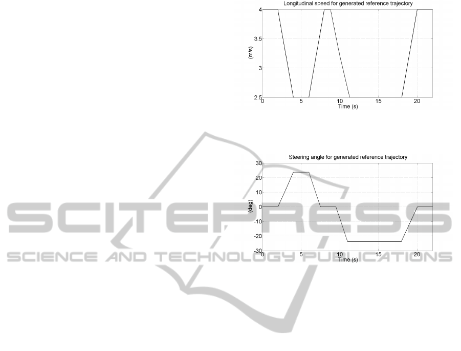
The generated reference trajectory based on a kine-
matic car-like vehicle model has received the speed
and the steering angle inputs depicted in Figures 3 and
4. The objective is to describe an usual trajectory for
small turn radius and not to test the capacities of the
passenger vehicle at the limits of handling. Hence, the
speed is reduced during the turn and the turn-around.
The maximum steering angle is 25
◦
and the steering
Figure 3: Input speed signal for the generated reference tra-
jectory.
Figure 4: Input steering angle for the generated reference
trajectory.
angle variation is less than 25
◦
/s which is comfort-
able during a standard driving in this range of speeds.
The comparison between the two simulation sce-
narios is motivated by the differences between the
kinematic car-like robot and the vehicle passenger
model, differences that are induced primary by the
slip of the tires. To do this comparison possible, pa-
rameters recorded for the two scenarios are displayed
mostly in the same figures. Figures 5 and 6 show the
trajectories followed by the car-like robot (model A)
and by the passenger vehicle (model B) with respect
to the reference car-like robot. The response for the
model A and B are very similar and satisfactory. The
initial error is corrected and the trajectory tracking
control succeeds for the turn-around.
The path-tracking errors are visible in Figure 7. At
the beginning, the error increases in order to change
the heading towards the reference trajectory but sub-
sequently the tracking is carried out with decreasing
error. A difference is visible between model A and B
during the turn-around, around t = 15s. The tracking
error increases for model B up to 0.8m. This differ-
ence can came from the tires deformation in curva-
ture. The longitudinal slip of the four tires for model
B is shown in Figure 8 while the side slip angles are
visible in Figure 9. The values recorded during curva-
tures are up to 10% for the longitudinal slip and up to
4
◦
for the side slip angles, which are moderate values
ICINCO2012-9thInternationalConferenceonInformaticsinControl,AutomationandRobotics
44

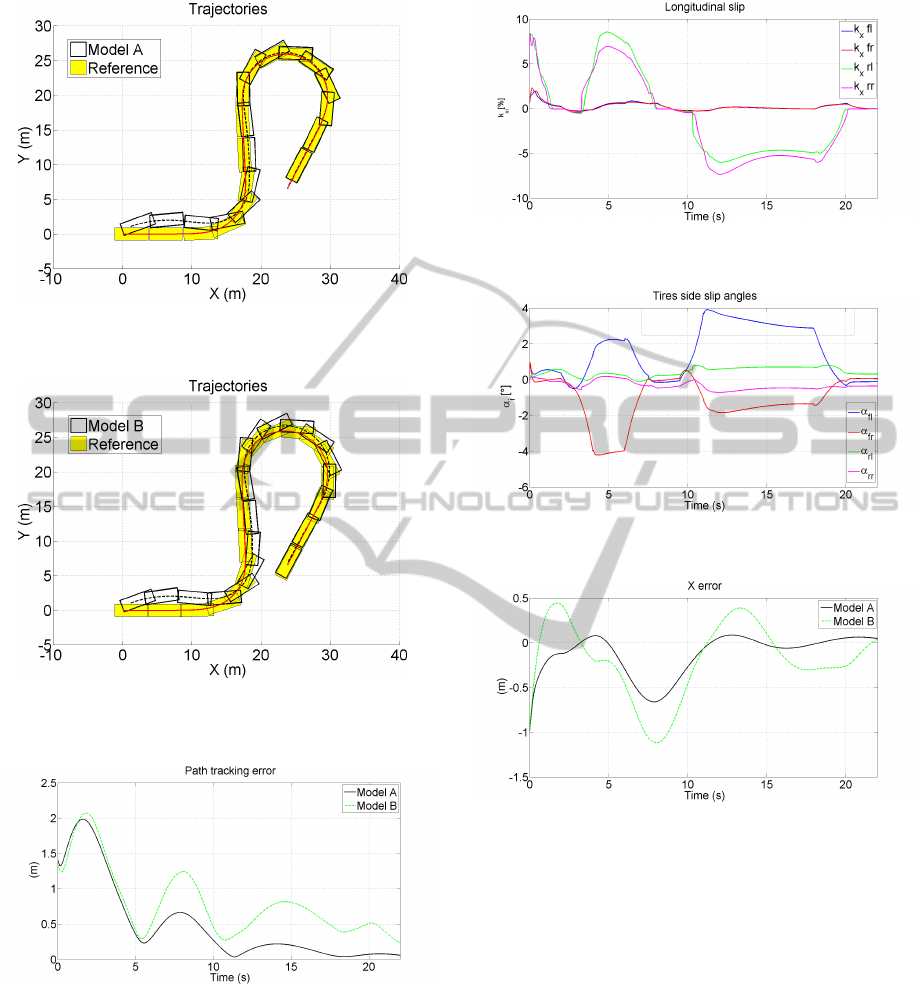
Figure 5: Trajectory of the model A with respect to the ref-
erence car-like robot.
Figure 6: Trajectory of the model B with respect to the ref-
erence car-like robot.
Figure 7: Path tracking error.
but sufficient to decrease the performance of model B
with respect to model A.
The relative errors with respect to the required tra-
jectory are presented in Figures 10 and 11 for the po-
sitions x and y and in Figure 12 for the longitudinal
speed. The most interesting is the error in lateral di-
rection. During the turn-around, this has very reduced
value below 0.2m for model A, while there are val-
ues up to 0.8m for model B. At the same time, the x
Figure 8: Longitudinal slip of the tires.
Figure 9: Side slip angles of the tires.
Figure 10: X error.
error is very reduced, close to zero. Hence, the path
tracking error comes mainly from the lateral error dur-
ing the turn around. The longitudinal speed is very
well followed by model A and with a consistent de-
lay for the passenger vehicle. This is explained by the
absence of the model for longitudinal dynamics for
model A, which has only a limitation of the accelera-
tion to ±4m/s
2
.
The evolution of the yaw rate of models A and B
with respect to the reference yaw rate is shown in Fig-
ure 13. This parameter is very satisfactory for both
models having a good following. The steering an-
gles are depicted in Figure 14. There is no saturation
necessary for both cases and the steering signal curve
is smooth enough to be followed by the actuator of
model B.
In Figures 15 and 16 the variation of the control
TrajectoryTrackingControlbyLMI-basedApproachforCar-likeRobots
45

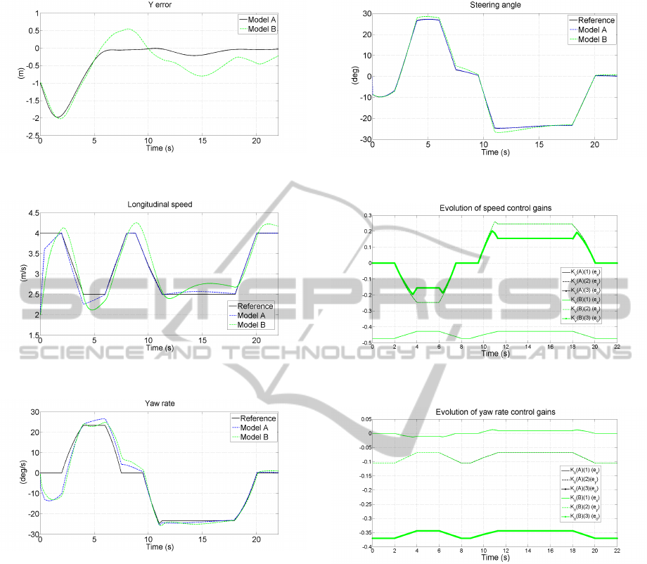
Figure 11: Y error.
Figure 12: Longitudinal speed error.
Figure 13: Yaw rate.
gains for the speed control input and for the yaw rate
input are shown. Identical signals can be noticed for
models A and B.
5 CONCLUSIONS
The work presented in this article investigates an LMI
based control approach to do trajectory tracking for
car-like robots. The approach needs an off line LMI
optimization and a computation of a 3 equations and
4 unknown variables system in real time. Developed
initially for an unicycle by (Gonzalez et al., 2009),
this control technique is completed with LMI con-
straints to make possible to use it on car-like robots
and implicitly on passenger vehicles. Moreover, the
method in this article takes into account poles place-
Figure 14: Steering angles.
Figure 15: Speed control gains.
Figure 16: Yaw rate control gains.
ment constraints. A preliminary study in simulation
is performed in order to estimate the possibility of
using this control technique on real passenger vehi-
cles. The trajectory tracking control is compared for
a car-like robot and for a complex modeled passen-
ger vehicle. The result is satisfactory and show the
feasibility of the concept. More investigations will
be conducted in the near future, including trajectory
tracking of recorded trajectories and comparison with
less complex control techniques, for instance the pure
pursuit approach.
REFERENCES
Boyd, S., Ghaoui, L. E., Feron, E., and Balakrishnan, V.
(1994). Linear Matrix Inequalities in System and Con-
ICINCO2012-9thInternationalConferenceonInformaticsinControl,AutomationandRobotics
46

trol Theory. Society for Industrial and Applied Math-
ematics.
Brault, P., Mounier, H., Petit, N., and Rouchon, P. (2000).
Flatness based tracking control of a manoeuvrable ve-
hicle: the pcar. In Proceedings of the Fourteenth Inter-
national Symposium of Mathematical Theory of Net-
works and Systems.
Brockett, R., Millman, R., and Sussman, H. (1983). Differ-
ential Geometric Control Theory. Birk ¨auser, Boston-
Basel-Stuttgart.
Campbell, S. F. (2007). Steering control of an autonomous
ground vehicle with application to the darpa urban
challenge. Master thesis, Massachusetts Institute of
Technology, USA.
Chilali, M. and Gahinet, P. (1996). H
∞
design with pole
placement constraints: An lmi approach. IEEE Trans-
actions on Automatic Control, 41(3):358–367.
DeLuca, A., Oriolo, G., and Samson, C. (1998). Feed-
back control of a nonholonomic car-like robot. Robot
Motion Planning and Information Sciences, 299:171–
253.
Enache, N. M., Mammar, S., Glaser, S., Lusetti, B., and
Nouveliere, L. (2009). Composite lyapunov based ve-
hicle longitudinal control assistance. In Proceedings
of the European Control Conference.
Enache, N. M., Mammar, S., Netto, M., and Lusetti, B.
(2010). Driver steering assistance for lane departure
avoidance based on hybrid automata and on composite
lyapunov function. IEEE Trans. on Intelligent Trans-
portation Systems, 11(1):28–39.
Falcone, P., Borrelli, F., Asgari, J., Tseng, H., and Hrovat,
D. (2007). Predictive active steering control for au-
tonomous vehicle systems. IEEE Transactions on
Control System Technology, 15:566–580.
Gonzalez, R., Fiacchini, M., Alamo, T., Guzman, J., and
Rodriguez, F. (2009). Adaptive control for mobile
robot under slip conditions using lmi-based approach.
In Proceedings of the European Control Conference.
Gonzalez, R., Fiacchini, M., Alamo, T., Guzman, J. L.,
and Rodriguez, F. (2010). Adaptive control for a mo-
bile robot under slip conditions using an lmi-based ap-
proach. European Journal of Control, 16:144–158.
Grant, M. and Boyd, S. (2011). CVX: Matlab software
for disciplined convex programming, version 1.21.
../../cvx.
Kim, B. and Tsiotras, P. (2002). Controllers for unicycle-
type wheeled robots: Theoretical results and experi-
mental validation. IEEE Transactions on Robotics and
Automation, 18(3):294–307.
Leedy, B. M., Putney, J. S., Bauman, C., Cacciola, S., Web-
ster, J. M., and Reinholtz, C. F. (2006). Virginia tech’s
twin contenders: A comparative study of reactive and
deliberative navigation. Journal of Field Robotics,
23(9):709–727.
Levinson, J., Askeland, J., Becker, J., Dolson, J., Held, D.,
Kammel, S., Kolter, J. Z., Langer, D., Pink, O., Pratt,
V., Sokolsky, M., Stanek, G., Stavens, D., Techman,
A., Werling, M., and Thrun, S. (2011). Towards fully
autonomous driving: Systems and algorithms. In Pro-
ceedings of the IEEE Intelligent Vehicles Symposium.
Li, L., Wang, F.-Y., and Zhou, Q. (2005). An lmi approach
to robust vehicle steering controller design. In Pro-
ceedings IEEE ITS Congress.
L¨ofberg, J. (2004). Yalmip : A toolbox for modeling and
optimization in MATLAB. In Proceedings of the
CACSD Conference, Taipei, Taiwan.
Mammar, S. and Yacine, Z. (2012). Invariant set based vari-
able headway time vehicle longitudinal control assis-
tance. In Proceedings of the American Control Con-
ference.
Mattingley, J. and Boyd, S. (2010). Real-time convex opti-
mization in signal processing. IEEE Signal Process-
ing Magazine, 27(3):50–61.
Michałek, M. and Kozłowski, K. (2011). Feedback con-
trol framework for car-like robots using unicycle con-
trollers. Robotica (in press), pages 1–19.
Minoiu, N., Mammar, S., Glaser, S., and Lusetti, B. (2010).
Vehicle assistance for lane keeping, lane departure
avoidance and yaw stability. approach by simultane-
ous steering and differential braking. Journal Eu-
rop´een des Syst`emes Automatis´es, 44(7):811–851.
Minoiu, N., Netto, M., Mammar, S., and Lusetti, B. (2009).
Driver steering assistance for lane departure avoid-
ance. Control Engineering Practice, 17(6):642–651.
Mnif, F. (2004). Recursive backstepping stabilization of a
wheeled mobile robot. International Journal of Ad-
vanced Robotic Systems, 1:287–294.
Montes, N., Mora, M., and Tornero, J. (2007). Trajec-
tory generation based on rational bezier curves as
clothoids. In IEEE Proceedings of the Intelligent Ve-
hicles Symposium.
Morin, P. and Samson, C. (2009). Control of nonholonomic
mobile robots based on the transverse function ap-
proach. IEEE Transaction on Robotics, 25(5):1058–
1073.
Oelen, W. and van Amerongen, J. (1994). Robust track-
ing control of two-degrees-of-freedom mobile robots.
Control Engineering Practice, 2(2):333–339.
Rajamani, R. (2006). Vehicle Dynamics and Control.
Springer Verlag, New York.
Scherer, C. and Weiland, S. (2004). Course on Linear Ma-
trix Inequalities in Control. Dutch Institute of Systems
and Control (DISC).
Snider, J. M. (2009). Automatic steering methods for au-
tonomous automobile path tracking. Technical report
cmu-ri-tr-09-08, Robotics Institute Carnegie Mellon
University Pittsburgh, Pennsylvania, USA.
Zhu, Y. (2008). Constrained nonlinear model predictive
control for vehicle regulation. Phd thesis, The Ohio
State University, USA.
TrajectoryTrackingControlbyLMI-basedApproachforCar-likeRobots
47