
Optimizing Operation Costs of the Heating System of a Household
using Model Predictive Control Considering a Local PV Installation
Cosmin Koch-Ciobotaru
1
, Fridrik Rafn Isleifsson
2
and Oliver Gehrke
2
1
Automation and Applied Informatics, Politehnica University of Timisoara, Blv. Parvan 2, Timisoara, Romania
2
Intelligent Energy Systems, Technical University of Denmark, Frederiksborgvej 399, Roskilde, Denmark
Keywords: Model Predictive Control, Optimization, Cost Minimization, Dynamic Thermal Storage, PV Penetration.
Abstract: This paper presents a model predictive controller developed in order to minimize the cost of grid energy
consumption and maximize the amount of energy consumed from a local photovoltaic (PV) installation. The
usage of as much locally produced renewable energy sources (RES) as possible, diminishes the effects of
their large penetration in the distribution grid and reduces overloading the grid capacity, which is an
increasing problem for the power system. The controller uses 24 hour prediction data for the ambient
temperature, the solar irradiance, and for the PV output power. Simulation results of a thermostatic
controller, a MPC with grid price optimization, and the proposed MPC are presented and discussed.
1 INTRODUCTION
The main issue (Vandoorn, 2011) is that the
electrical distribution grid was not designed for bi-
directional power flow, i.e. that power would not
only flow to the lower voltage levels where most
consumer are connected, but that it could also flow
“up” to the higher voltage levels.
The increased amount of PV plants in the
distribution grid introduces some complications,
such as the fluctuating nature of PV production
which has limited predictability (Madureira, 2009).
There are fast fluctuations, due to cloud transients,
which cause problems with voltage regulation. There
are also slower fluctuations due to the movement of
the sun and changes in cloud cover, so if the PV
plant generation is not coordinated with the local
consumption it might be necessary to invest in more
grid capacity as presented in (Ueda, 2007).
In the distribution grid there is also a foreseeable
increase in new types of loads, such as heat pumps
and electric vehicles, both loads that can to some
degree act as flexible loads as shown in
(Madureira,2009).
If loads that are flexible can be intelligently
managed, it could be possible to help the distribution
grids to cope with both increased renewable
production and increased loads. Furthermore, this
intelligent control could also reduce the need for
expensive grid extensions if loads and production
are coordinated locally.
This control is seeking to incorporate predictions
of weather, occupancy behaviour, renewable energy
availability, and price signals from the grid. The
model predictive control (MPC) presents a
methodology that can use all these predicted values
in order to improve the energy efficiency
consumption by load shifting and peak shaving,
minimize the cost of operation by using low price
energy, as shown in (Nagai, 2002) and in (Ma 2011),
and maximizing the use of renewable energy.
This paper proposes a MPC that minimizes the
overall electrical energy cost of heating a building
which also has a local PV installation. By using the
buildings ten 1 kW heaters, a price signal for
electrical energy, a prediction of solar irradiation, of
PV output power, and of ambient temperature it is
possible to coordinate the heaters consumption so
that as much energy as possible is consumed from
the locally produced PV.
2 MODEL OF THE SYSTEM
Model predictive control uses a model of the system
in order to predict the process output over a future
horizon of N time steps and solves a quadratic
optimization problem with the control signal as the
decision variable. In addition, constraints can be
formulated both for manipulated and controlled
431
Koch-Ciobotaru C., Rafn Isleifsson F. and Gehrke O..
Optimizing Operation Costs of the Heating System of a Household using Model Predictive Control Considering a Local PV Installation.
DOI: 10.5220/0004054804310436
In Proceedings of the 2nd International Conference on Simulation and Modeling Methodologies, Technologies and Applications (SIMULTECH-2012),
pages 431-436
ISBN: 978-989-8565-20-4
Copyright
c
2012 SCITEPRESS (Science and Technology Publications, Lda.)

variables as formulated in (Huusom, 2010) and
(Oldewurtel, 2010).
The model used in this paper is extensively
presented in (Bacher, 2010) and represents a house
of approximately 125 m
2
divided between eight
rooms. Every room is equipped with heaters: two
rooms have two heaters and the others have one
heater each. The heaters are considered to have the
output power of 1kW.
The model approximates the interior of the
building to be one room with a uniform inside
temperature. The state variable is the inside
temperature (T
i
), the input is the power to the heaters
(P
H
) and the disturbances are the solar irradiance (G)
and the ambient temperature (T
a
).
The temperature dynamics of a given space can
be modelled using a resistance-capacitance (RC)
circuit analogy, see figure 1, and formulated as a
linear state space model.
(a) (b)
Figure 1: Thermal dynamic model of the house.
(1)
Where C
i
is the heat capacity of the house. This
includes the indoor air and the interior objects
(=3.42 [kW/°C])
R
ia
is the thermal resistance from the indoor to
the ambient environment (=4.87 [°C/kW])
A
w
is the effective window area of the house
with heating influence (=5.53 [m
2
])
3 OFFSET FREE MPC
The predicted disturbances values that are available
to the model usually present an error compared to
the real measured values. In order to eliminate the
offset caused by these differences, filters have to be
implemented for each of the predicted values fed
into the controller. In this way, the controller will
not track the predicted values, but their variations.
This gives, compared to Equation 1, an extended
state space model with an additional state for each
filtered variable:
(2a)
(2b)
For simplification, we introduce the new state
model on the basis of equation 3:
(3a)
(3b)
The usage of a Kalman filter in the algorithm
consists of two stages that run cyclically:
- Time update – responsible for projecting the
state ahead
(4)
- Measurement update – which has the role to
‘correct’ the estimated values by considering the
measurements taken from the system
(5)
The covariance P is a symmetric positive
semidefinite solution of the discrete Ricatti equation:
(6)
The covariance of the innovations R
e
and the
predictive Kalman gain K
f
are computed using
equations 7 and 8:
(7)
(8)
The simulation uses the quadprog solver from
Matlab for which the optimization problem has to be
rewritten in the form of Equation 9:
(9)
Subject to
(10)
The model output for the predicted horizon of N
time steps is:
(11)
Equation 4 has the following coefficients:
(12)
(13)
Where
(14)
SIMULTECH 2012 - 2nd International Conference on Simulation and Modeling Methodologies, Technologies and
Applications
432

In this case, the result of the MPC optimization
problem is the difference ∆u
k
and the command to
the system is u
k
= u
k-1
+ ∆u
k
.
4 SIMULATION SCENARIOS
In all the simulations the MPC controller uses the
model described in Equation 2.
These two additional state variables are used for
implementing the filter in order to achieve offset
free control in the presence of deviations from the
predicted values of the two disturbances.
The MPC controller has hard limitations on the
controlled variable – the inside temperature, that has
to be inside [20...22]°C interval and on the
manipulated variable – power supplied to the
heaters, that has to be in the [0...10] kW interval, and
can have only integer as power steps.
The MPC controller starts with offline predicted
values for solar irradiance, temperature, and grid
price and for the third simulation case, the predicted
PV power output.
The time step of the simulations is 10 minutes,
and the prediction horizon is 80 time steps.
During each simulation, two different cases can
be studied:
- The first, when the house does not have any PV
installation – the heaters are consuming power
entirely from the grid
- The second, when the house has a PV
installation – the heaters are consuming power both
from the PV plant and from the grid. The higher
priority is to consume from the local PV plant and
the remaining required power is taken from the grid.
The amount of unused PV energy is sold to the grid.
4.1 Simulation Scenario 1
A thermostatic controller is implemented to maintain
the temperature inside given limits: [19.2...21]. For
comparison reasons, the limits in this simulation
scenario differ from the other two scenarios in order
that the average temperature in the house, for the
simulation time, to be the same. This has the purpose
to accurately reflect the MPC controller’s effect in
similar operation conditions.
4.2 Simulation Scenario 2
The MPC tracks the inside temperature with
minimal overall energy cost. The controller is
considering all the energy to be taken from the grid,
at a market imposed price (C
G
).
The optimization function is represented by
Equation 15:
(15)
4.3 Simulation Scenario 3
The MPC controller tracks the inside temperature
with minimal overall energy cost, also considering
the power production of the installed PV panels. The
controller calculates a virtual price on which the
available PV power, that has a lower cost for the
user (C
PV
) of 0.02 Euros, is considered to alter, with
a weight factor, the market imposed price.
(16)
The cost minimization function would be
(17)
Considering U as the optimization variable and
replacing 16 in 17 the equation 18 is obtained:
(18)
Where C
G
– is the predicted price of the grid
energy
U – represents the vector with the next N
command values for the time horizon
P
PV
– represents the predicted output power from
the PV installation
(19)
Where additional assumptions were made:
-
- a weight factor
- at each optimization step, u
s
is taken as the
last command value, u
k-1
.
The optimization function is written as:
(20)
5 RESULTS
Results from the three simulation scenarios are
presented in Figures 2 to 4 and compared in Table 1,
where the following notations have been used:
Optimizing Operation Costs of the Heating System of a Household using Model Predictive Control Considering a Local PV
Installation
433
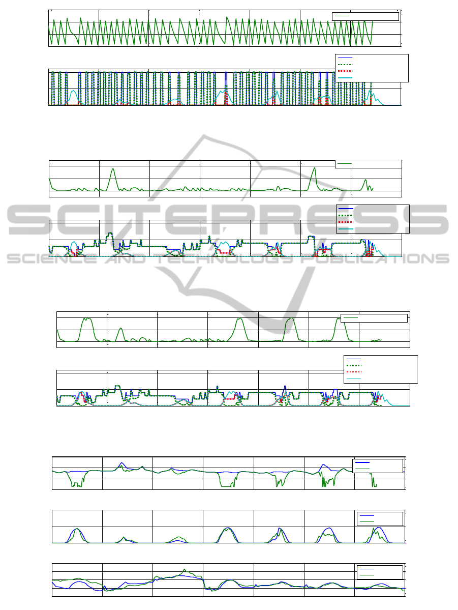
Figure 2: Thermostatic control.
Figure 3: MPC with grid price optimization.
Figure 4: MPC with virtual price optimization considering PV power output prediction.
Figure 5: Data used by controllers: price values, predicted and measured ambient data.
24 48 72 96 120 144 168
19
20
21
22
Inside temperature (
0
C)
t (hours)
Inside Temperature (
0
C)
24 48 72 96 120 144 168
0
5
10
Power
t (hours)
Power (kW)
Power for Heaters
Power from Grid
Power from PV
PV power generation
Inside temperature
24 48 72 96 120 144 168
20
21
22
Inside temperature (
0
C)
t (hours)
Inside Temperature (
0
C)
24 48 72 96 120 144 168
0
5
10
Power
t (hours)
Power (kW)
Power for Heaters
Power from Grid
Power from PV
PV power generation
Inside temperature
24 48 72 96 120 144 168
20
21
22
Inside temperature (
0
C)
t (hours)
Inside Temperature (
0
C)
24 48 72 96 120 144 168
0
5
10
Power
t (hours)
Power (kW)
Power for Heaters
Power from Grid
Power from PV
PV power generation
Inside temperature
24 48 72 96 120 144 168
0
0.02
0.04
0.06
Price
t (hours)
Price (Euros/kWh)
24 48 72 96 120 144 168
0
0.5
1
Solar irradiance
t (hours)
Solar irradiance (kW/m
2
)
24 48 72 96 120 144 168
-5
0
5
10
15
Ambient temperature
t (hours)
Ambient temperature (
0
C)
Real price
Virtual price
Predicted
Measured
Predicted
Measured
SIMULTECH 2012 - 2nd International Conference on Simulation and Modeling Methodologies, Technologies and
Applications
434

Table 1: Energy consumption and cost results from simulations.
Sim.
ID
Config.
Type
E
H
(kWh)
E
PV2H
(kWh)
E
G2H
(kWh)
E
PV
(kWh)
E
PV2G
(kWh)
C
G2H
(Euros)
C
PV2H
(Euros)
Avg Ti
(°C)
Simulation 1, with thermostatic controller around 20.14°C
S
11
No PV
496.66
-
496.66
-
-
16.75
-
20.14
S
12
PV
496.66
21.68
474.98
110.58
88.90
15.98
0.43
20.14
Simulation 2, with grid price optimization
S
21
No PV
496.66
-
496.66
-
-
16.61
-
20.14
S
22
PV
496.66
71.01
425.65
110.58
39.57
14.12
1.42
20.14
Simulation 3, with grid price and PV availability
S
3
PV
500.8
94.37
406.4
110.08
16.21
13.57
1.88
20.34
Sim. ID – simulation identifier
Config. Type – type of house configuration: with
or without PV installation
E
H
– the total energy consumed by the heaters
during simulation interval
E
PV2H
– the amount of energy consumed by the
heaters from the local produced PV energy
E
G2H
– the amount of energy consumed by the
heaters from the grid
E
PV
– the amount of energy produced by the PV
installation
E
PV2G
– the amount of energy produced by the
PV to be sold to the grid
C
G2H
– cost of E
G2H
in Euros
C
PV2H
– cost of E
PV2H
in Euros
Avg. Ti – average inside temperature over the
simulated time horizon
The grid energy prices are shown in the first plot
from Figure 5. It is assumed that the predicted grid
energy prices coincide with the actual ones. In the
same figure, the virtual price used during Simulation
3 is also plotted.
During simulations S
1x
and S
2x
the controller
does not present information regarding the presence
of an PV installation and acts according only to
signals available for each case, as stated in section 3.
Achieving the same average inside temperature
implies the same amount of energy is used. As the
ambient temperature and the solar irradiance are the
same for each simulation, the amount of electric
energy used to keep the inside temperature is the
same. The difference is represented by the heaters
consumption shifting according to the used
controller.
In S
1x
a thermostatic controller is used, as
presented in section 3. It can be seen that during
clear days, with large solar irradiance values, the
heaters are turned off most part of the day, the
thermal energy being largely taken from the ambient
factors. In S
12
only 21.68 kWh, representing around
20% of the available PV local produced energy, is
consumed from the PV.
In S
2x
the MPC with grid price optimization is
used. The same amount of electric energy is used as
in S
1x
, for achieving the same inside temperature.
However, the MPC shifts the heaters’ consumption
to low price moments, and stores thermal energy
before price peaks as it can be seen in Figure 3,
before the energy price peaks at time 200 and 780,
shown in Figure 5.
The MPC controller from S
2x
achieves a cost
reduction from 16.75 to 16.61 Euros in the case of
S
21
and from 15.98 to 14.12 in the case of using a
PV installation of S
22
. In S
22
, 71.01 kWh of local PV
energy is consumed, representing 64% of the PV
production.
However, the local PV energy usage for S
12
and
S
22
are unpredictable since the controller does not
consider the PV production.
In S
3
the MPC’s objective is to consume as much
locally produced energy as possible. This is realized
by implementing the virtual price, presented in
section 3, in the optimization function. Figure 4
depicts the operation of the MPC which uses the
house’s thermal capacity to store the local PV
energy during large solar irradiance values.
In this case, the cost of the energy consumed
from the grid is 13.57 Euros and 85% of the local
PV produced energy is consumed.
6 CONCLUSIONS
The paper emphasises the benefits of using model
predictive control for houses as dynamic thermal
energy storage.
By formulating the correct optimization
problems and feeding the controller with predictions
on the system’s variables, the MPC is able to
achieve cost reduction on the electrical energy
consumption from the grid.
As demonstrated through simulations in this
paper, the MPC can consider the presence of an
Optimizing Operation Costs of the Heating System of a Household using Model Predictive Control Considering a Local PV
Installation
435

installed PV plant maximizing the usage of locally
produced renewable energy. The consumption of
locally produced energy has a major benefit both for
the user, by lowering the overall cost of energy and
also for the operation of distribution grids with a
high penetration of renewable energy generation.
This paper presented an algorithm that deals with
the two problems: minimizing the operating cost of
the house heating system and maximizing the use of
local produced energy and lowering the burden on
the distribution grid.
From the source of power consumption
perspective, the algorithm can be extended to use the
energy from other types of local renewable energy
sources. It can be extended also from the perspective
of the types of loads that are shifted, not focusing
only on the heat system but also on different
household appliances.
The proposed algorithm can be used to manage
energy produced by other types of renewable energy
generation, such as wind turbines and combined heat
and power plants. The algorithm can also be
modified for other types of consumption that has the
ability to be shifted in time, such as water heaters,
air conditioning units and refrigeration systems.
ACKNOWLEDGEMENTS
This work was supported in part by the strategic
grant POSDRU/88/1.5/S/50783 (2009) of the
Ministry of Labor, Family and Social Protection,
Romania, co-financed by the European Social Fund
– Investing in people and also partially supported by
the E.U. Project No. 228449/2011.
REFERENCES
Bacher P., Thavlov A., Madsen H., Models for Energy
Performance Analysis, IMM-Technical Report-2010-
02.
Huusom J. K., Poulsen N. K. , Jørgensen S. B. and
Jørgensen J. B., 2010, Tuning of Methods for Offset
Free MPC based on ARX Model Representations. In
American Control Conference, ACC 2010, 30 June -02
July 2010 in Baltimore, USA.
Ma Y., Anderson G., Borrelli F., A Distributed Predictive
Control Approach to Building Temperature
Regulation. In American Control Conference, ACC
2011, 29 June – 01 July, 2011 in San Francisco, USA.
Madureira A. G. and Lopes J. A. P., Coordinated voltage
support in distribution networks with distributed
generation and microgrids. In IET Renewable Power
Generation, vol. 3, no. 4, pp. 439–454, Dec. 2009.
Nagai T., Optimization Method for Minimizing Annual
Energy, peak energy demand, and annual energy cost
through use of building thermal storage, ASHRAE
Transactions, vol. 108, no. 1, pp. 976-887, 2002.
Oldewurtel F., Parisio A., Jones C. N., Morari M.,
Gyalistras D., Gwerder M., Stauch V., Lehmann B.,
Wirth K., Energy Efficient Building Climate Control
using Stochastic Model Predictive Control and
Weather Predictions. In American Control
Conference, ACC 2010, 30 June -02 July 2010
Baltimore, USA.
Pannochia G. and Rawlings J., Disturbance Models for
Offset-Free Model Predictive Control. In AIChE
Journal 2003, Volume 49, Issue 2, pp. 426-437.
Ueda Y., Kurokawa K., Tanabe T., Kitamura K.,
Akanuma K., Yokota M., Sugihara H., Study On The
Over Voltage Problem And Battery Operation For
Grid-Connected Residential PV Systems. In 22nd
European Photovoltaic Solar Energy Conference, 3-7
September 2007, Milan, Italy
Vandoorn T. L., Renders B., Degroote L., Meersman B.,
and Vandevelde L., Active Load Control in Islanded
Microgrids Based on the Grid Voltage. In IEEE
Transactions on Smart Grid, Vol. 2, No. 1, pp. 139-
151, 2011
SIMULTECH 2012 - 2nd International Conference on Simulation and Modeling Methodologies, Technologies and
Applications
436
