
Direct Numerical Simulation of Flow Past a Sphere in a Plane
Turbulent Boundary Layer with Immersed Boundary Method
Hui Zhao, Anyang Wei, Kun Luo and Jianren Fan
State Key Laboratory of Clean Energy Utilization, Zhejiang University, Hangzhou, China
Keywords: Direct Numerical Simulation, Immersed Boundary Method, Boundary Layer, Sphere, Plane.
Abstract: Direct Numerical Simulation coupled with Immersed Boundary Method (IBM) has attracted wide atten-
tion recent years, making this technique a significant role in many practical engineering areas. This paper
described a direct numerical study of flow past a sphere above a plane, which can obtain detail infor-
mation of flow field and vortex structure. A combined multiple-direct forcing and immersed boundary
method (MDF/IBM) was used to deal with the coupling between fluid and solid. The Reynolds number
based on sphere diameter was 4171. Behaviours of the vortices were observed through the simulation. The
velocity distribution switched from laminar boundary to turbulent boundary. A recirculation region was
observed behind the sphere. The influence of the sphere on the boundary layer, the center peak defect, the
turbulence intensity and the Reynolds stresses are explored.
1 INTRODUCTION
A number of studies have been carried out on a flow
pasting a three-dimensional obstacle placed on the
plane boundary, especially the flow past a sphere.
Obtaining enough data and understanding the struc-
ture of flow field and vortex are extremely necessary.
Because from an engineering viewpoint, the spheri-
cal structure application can be seen everywhere in
practice, such as some structures exposed in the
wind, vehicles moving in fluid and so on. After
Schlichting studied a blunt obstacle placed on the
plane boundary with the effect of surface roughness
(Schlichting, 1939), the drag of a sphere placed on a
ground plate (Klemin et al., 1939) was investigated.
An experimental study of the turbulent shear layer
behind a sphere placed on a plane boundary was
performed (Okamoto, 1980). The surface pressure
distribution on a sphere, the velocity and pressure
distribution in the shear layer behind a sphere were
measured. It was found that the wall wake behind a
sphere became low and spreads transversely with the
downstream distance increasing. Takayuki (Taka-
yuki, 2008) investigated the flow around a sphere
placed at various heights above a plane boundary. In
Takayuki’s experimental study, the surface pressure
distribution on the sphere and the plane were meas-
ured, meanwhile empirical equations of the drag and
lift coefficients were defined.
In recent years, with the development of the
computer technology, it becomes possible to do
research on two-phase flow in turbulent boundary
layer using direct numerical simulation method.
Fully resolved direct numerical simulations were
considered to investigate a turbulent channel flow
over an isolated particle of finite size (Zeng et al.,
2008) with the spectral element methodology (SEM).
To validate a joint application of direct numerical
simulation and a combined multiple-direct forcing
and immersed boundary method (MDF/IBM), a flow
past an isolated three-dimensional hemispherical
roughness element mounted on a flat plate was
simulated (Zhou et al., 2010). Nevertheless,
numerical simulation studies on the interaction
between sphere and plane boundary layer are
lacking, which could be significant to engineering
application.
This paper describes a direct numerical study on
the flow field and the vortex structure on a sphere
above a plane. The influence of the sphere on the
boundary layer is explored, such as velocity
distribution, turbulence intensity, Reynolds stresses
and vortex structure.
243
Zhao H., Wei A., Luo K. and Fan J..
Direct Numerical Simulation of Flow Past a Sphere in a Plane Turbulent Boundary Layer with Immersed Boundary Method.
DOI: 10.5220/0004056802430249
In Proceedings of the 2nd International Conference on Simulation and Modeling Methodologies, Technologies and Applications (SIMULTECH-2012),
pages 243-249
ISBN: 978-989-8565-20-4
Copyright
c
2012 SCITEPRESS (Science and Technology Publications, Lda.)

2 NUMERICAL METHOD
2.1 Governing Equations
In the computational domain Ω, the dimensionless
governing equations for incompressible viscous
flows are:
(1)
(2)
Here, u is the dimensionless velocity of fluid, P is
the dimensionless pressure, Re is the Reynolds
number defined as
, where is the
characteristic density of fluid, U is the characteristic
velocity, L is the characteristic length of flow field
and is the viscosity of fluid.
2.2 Multi-direct Forcing Immersed
Boundary Method
Function f in the momentum equation (2) is the
mutual interaction force between fluid and
immersed boundary, this dimensionless external
force is expressed as:
(3)
where
is the Dirac-delta function.
is
the position of the kth Lagrangian point on the
immersed boundary. x is the position of the Eulerain
grid nodes.
is the force that exerts on the
fluid by the kth Lagrangian point of the immersed
boundary.
(4)
where
, and n, n+1
represent two different time.
Here,
is an intermediate variable which
satisfies the governing equations of the pure flow
field, then we can get
.
In order to ensure that the no-slip boundary con-
dition of the velocity at the immersed boundary
could be satisfied, Direct forcing (Mohd-Yusof,
1997) is introduced to make the velocity on the La-
grangian points approaching the velocity of the
no-slip boundary. Therefore the force exerted on the
kth Lagrangian point at the immersed boundary is:
(5)
If this direct forcing is exerted by l+1 times, the
intermediate velocity
could be much closer to
the desired velocity
.Then
could be
expressed as:
(6)
At the same time, to spread the force from the
Lagrangian points to the Eulerian grids, the two way
coupling between Lagrangian points and Eulerian
grids could be achieved through the Dirac delta
function. Then we can get the functions of the force
spread into the Eulerian grids, flow field and
velocity of the points on the immersed boundary.
When the Direct forcing is exerted by NF times
in a time step, the velocity at the immersed
boundary can get close enough to the desired
velocity under the no-slip condition. The interaction
force between fluid and Lagrangian points could be
described as :
(7)
The method mentioned above is called Multi-direct
Forcing (Luo et al., 2007); (Wang et al., 2008).
A closed-form expression for the velocity
distribution over a smooth wall is valid continuously
from the wall up to the freestream (Musker, 1979).
In this paper, it is applied to calculate the
streamwise velocity of the entrance velocity. And
the open boundary condition (Orlanski, 1976) is
applied as the convective velocity boundary
condition.
2.3 Computational Domain
The geometrical parameters of the domain are
X×Y×Z=74.55mm×14.1mm×10.5mm, which can be
seen in figure1, and the sphere center is placed at
O(16.35mm, 7.05mm, 1.8mm). The precision of
uniform grid is 50μm, thus the grid amount of the
whole flow field is 92,897,280. The domain is di-
vided into 48 subdomains, and the resolution along
the streamwise, spanwise and wall-normal directions
are 16×3×1. Parameters of the sphere and fluid are
SIMULTECH 2012 - 2nd International Conference on Simulation and Modeling Methodologies, Technologies and
Applications
244
set out in Table 1.
The size of the gap between the bottom of the
sphere and the plane is 0.1D, which is 0.3mm.
According to the expression
,
the amount of Lagrangian points (Uhlmann, 2005) is
9520, distances between any two points are equal in
length.
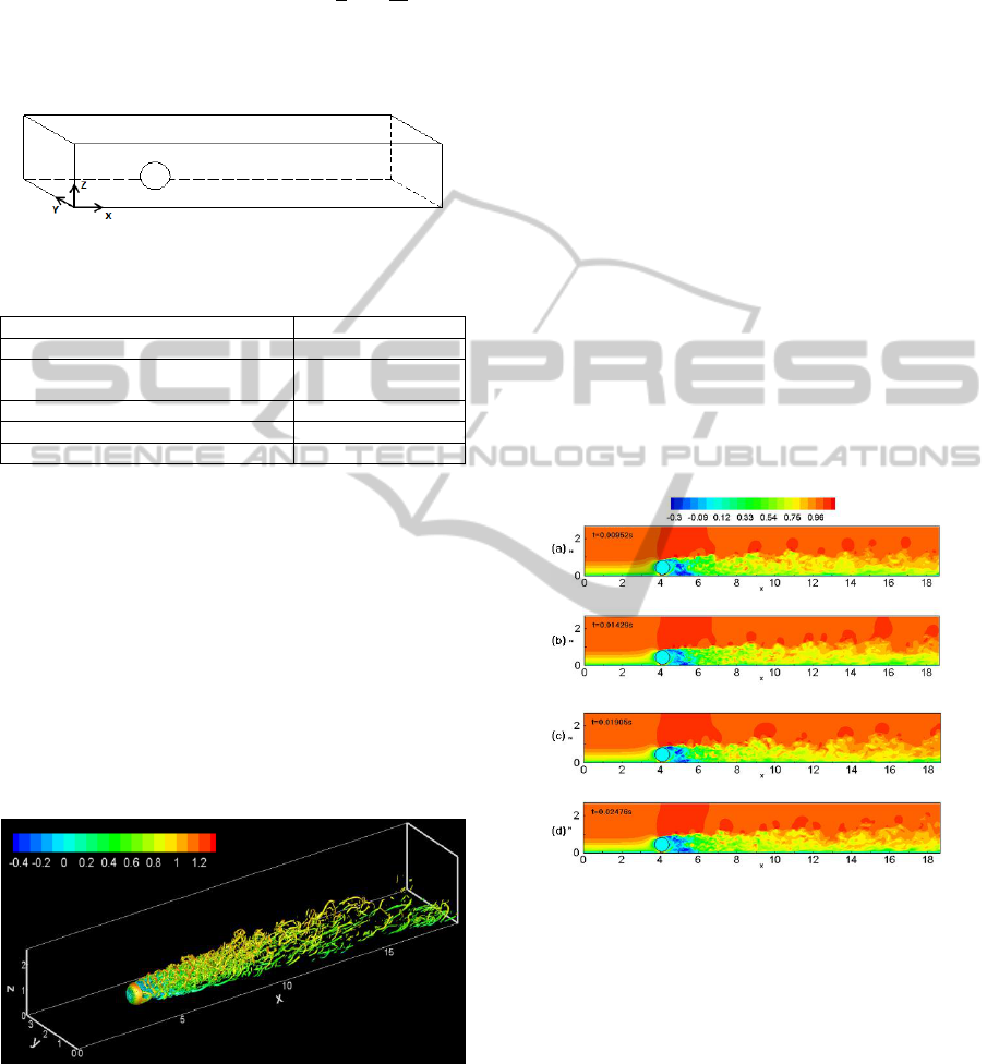
Figure 1: Schematic view of the computational domain.
Table 1: Summary of prediction conditions.
Parameter
value
Sphere diameter, D (mm)
3
Position of the sphere center,
O(x
o
mm,y
o
mm,z
o
mm)
(16.35 , 7.05 , 1.8)
Air density, ρ(kg/m3)
1.205
Air viscosity, μ (kg/m/s)
1.82×10
-5
Free stream velocity, U (m/s)
21
3 RESULTS AND DISCUSSION
According to the simulation results, we analyse the
structure of the vortex, the distribution of velocity
and pressure, the turbulence intensity, and so on.
The structure of the vortex is observed in figure
2, from which no horseshoe vortices and arch
vortices could be find, but hairpin vortex formed and
shed form the sphere, thus the forest vortices are
formed. It is consistent with the experimental results
of Takayuki (Takayuki, 2008).
Figure 2: Vortex structure of the entire domain.
The average velocity field in the center section
Y=y
o
at four different time steps are presented in
figure 3. The streamwise velocity distribution of the
boundary layer is visualized clearly. It can be seen
from the illustration that there is a typical laminar
flow velocity distribution in front of the sphere.
Then the flow is splited: the under part flows
through the gap between the sphere and the plane.
Because of the across area reducing suddenly, a high
velocity area is formed, extending to the
recirculation region behind the sphere. And the
upper part climbs upward along the sphere.
Boundary layer separation take place on the
separation point at the top of the sphere. The
separated boundary layer sharply thickens along the
flow, and under the separated boundary layer, a
recirculation region is formed behind the sphere.
The sharply thickening of the boundary layer
indicates the transition of the boundary layer. And
behind the transition zone, the profile of the
boundary layer velocity converts from the fully
developed laminar boundary layer to fully
developed turbulent boundary layer. According to
figure 3, the turbulent boundary layer develops
continuously with time, and the wake rises along the
normal direction. At the same time, the length of the
transition zone reduces. Laminar sublayer could be
distinguished from figure 3(c).
Figure 3: The streamwise velocity distribution of the
boundary layer, (a) t=0.00962s, (b) t=0.01429s, (c)
t=0.01905s,(d) t=0.02476s.
Figure 4(a) shows the profiles of the mean
velocity defect at X/D=10(X=x-x
o
). With the
vertical distance increasing, the peak velocity defect
decreases and almost vanishes at Z/D=0.8. And as
the upward distance increasing, its position closed to
the center when Z/D <0.6, yet moved away from the
center when Z/D >0.6. On the spanwise direction,
the velocity defect decreases faster when
Y/D>0.5(Y=y-y
o
) than the center behind the sphere.
Figure 4(b) indicates the mean velocity defect at
Z/D=0.6. In the range of Y/D<0.7, the peak defect is
Direct Numerical Simulation of Flow Past a Sphere in a Plane Turbulent Boundary Layer with Immersed Boundary Method
245
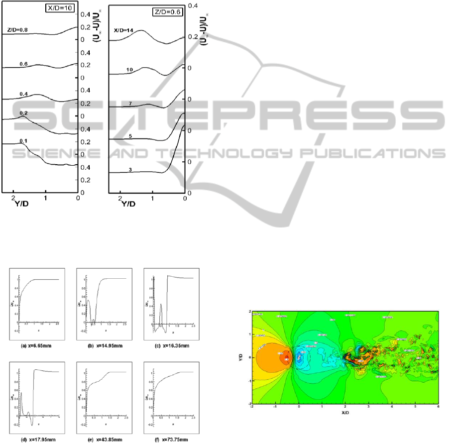
mainly affected by the recirculation region behind
the sphere. When the downstream distance increas-
ing, the center peak defect decreases, and another
peak velocity defect appears at X/D=7. The
spanwise peak defect shifts in the Y-direction,
which takes place at Y/D=1.1 for X/D=7 and at
Y/D=1.4 for X/D=14. Figure 5(a)-(f) shows the
profile of mean velocity at plane Y=y
o
.
(a)
(b)
Figure 4: (a) Profiles of mean velocity defect in the verti-
cal section X/D=10; (b) Profiles of mean velocity defects
in the horizontal centre section Z/D=0.6.
Figure 5: Profiles of mean velocity in the centre section
Y=y
o
. (a) x=6.65mm, (b) x=14.95mm, (c)x=16.35mm,
(d)x=17.95, (e) x=43.85mm, (f) x=73.75mm.
The dimensionless position of the sphere center
at Z-axis is 0.075. At x=6.65mm, a typical laminar
boundary layer velocity profile is presented as the
entrance velocity profile.In figure 5(b) fluctuations
in the range of 0.3<z<0.6, is the result of the IBM
method, not the velocity of fluid. According to the
IBM method, it is solid inside the sphere, which has
been computed as fluid. Thus the velocity is 0 in fact.
And the profile indicates that the existence of the
sphere “breaks” the laminar boundary layer velocity
profile. The mean velocity profile at the position of
the sphere center is observed in figure 5(c). Actually,
the fluctuation in the range of 0.075<z<0.825 is not
the velocity of fluid as well. Due to the influence of
the sphere, a high velocity area forms in the gap
between the sphere and the plane. In the range of
0.825<z<1.000 at the top of the sphere, a thin
boundary layer exists, where the dimensionless
velocity sharply increases from 0 to 1.2. Figure 5(d)
shows the mean velocity profile at 0.1mm behind
the sphere. Because of separation of the boundary
layer and the formation of the recirculation region,
mean velocity presents negative values. Figure 5(e)
and (f) respectively describes the profile at
x=43.84mm and x=73.75mm. The influence of the
sphere on the boundary layer is much weaker when
x equals to 73.75mm, and the velocity profile
indicates a typical turbulent layer velocity profile.
The pressure distribution on the plane can be
observed in figure 6. There are two areas of high
pressure respectively in front of the sphere and
behind the recirculation area. Behind the sphere, the
low pressure area which coincides with the
recirculation area is reduced rapidly because of a
strong downwash behind the sphere. Hence the
length of the recirculation region is considered to be
twice as much as the diameter of the sphere between
the two high pressure areas.
Figure 6: The pressure distribution on the plane.
In figure 7 the time-mean velocity profiles at
X/D=5~14 are presented. The thickness of boundary
layer is nearly equal to 1.8D at X/D=5, and thikens
with downstream distance increasing. The
turbulence intensity on X-component, Y-component
and Z-component are compared in figures 8-10.
Because of the existance of the sphere, the
SIMULTECH 2012 - 2nd International Conference on Simulation and Modeling Methodologies, Technologies and
Applications
246
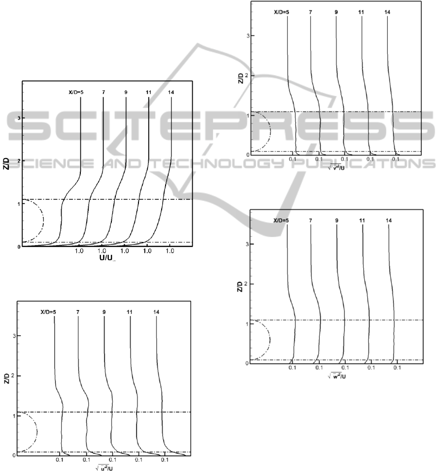
turbulence intensity values in the virtical direction is
divided into three zones natually. In the range of
0<z<0.075, turbulence intensity in X-direction and
Y-direction decreases rapidly with the virtical
distance increasing, but in Z-direction, it increases.
In the range of 0.075<z<0.825, turbulence
intensityis about 0.1 in all directons and decreases
with streamwise distance increasing. The value of
turbulence intensity gradually tends to the value of
freestream in the range of z>0.825, which
approaches zero. And the change is gentler as the
streamwise distance increasing. Thus it can be seen
that turbulence intensity is increase in the shear
layer.
Figure 7: Profiles of mean velocity in the centre section
Y=y
o
.
Figure 8: Profiles of turbulence intensity in X-direction in
centre section Y=y
o
.
Figure 11 shows the Reynolds stresses profile in the
plane Y=yo. At the position x=20.60mm, two peaks
which have different direction are presented
respectively at z=1mm and z=3.6mm. Similarly, at
other positions in the X-directon, two peaks in the
opposite direction exist. And with the increase of x,
peak values reduce, which is closed to zero near the
outlet of the computational domain where x equals
to 73.75mm.
Figure 9: Profiles of turbulence intensity in Y-direction in
centre section Y=y
o
.
Figure 10: Profiles of turbulence intensity in Z-direction in
centre section Y=y
o
.
The X-component, Y-component and
Z-component of the turbulence intensity in the
horizontal center section (Z/D=0.6) and the vertical
section where X/D=10 are shown in figures 12-13.
The position of peak of turbulence intensity moves
in a manner similar to peak velocity defect. While
Z/D<0.8, the turbulence intensity at the streamwise
is larger than the lateral and vertical turbulence
intensities. And at Z/D=1.2, the turbulence becomes
almost isotropic.
Direct Numerical Simulation of Flow Past a Sphere in a Plane Turbulent Boundary Layer with Immersed Boundary Method
247
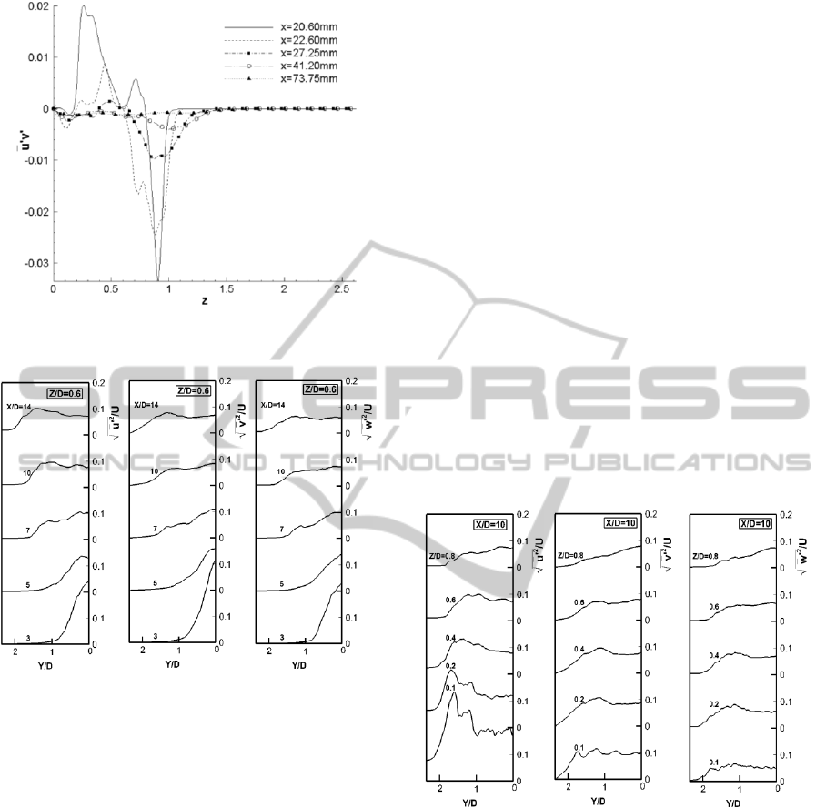
Figure 11: Profiles of Reynolds stress in the centre section
Y=y
o
.
(a)
(b)
(c)
Figure 12: Profiles of turbulence intensity in the horizontal
centre section (Z/D=0.6). (a) in X-direction; (b) in
Y-direction; (c) in Z-direction.
4 CONCLUSIONS
In this paper, we have studied the flow field around
a sphere placed above a ground plane. The gap be-
tween the sphere and the plane is 0.1D. The Reyn-
olds number based on D is 4171.The MDF/IBM
method has been used to deal with the coupling be-
tween fluid and solid. The main findings of this
study are summarized in the following.
(1) Hairpin vortex is formed and sheds behind the
sphere, and the forest vortices are formed.
(2) In front of the sphere there is a typical
laminar flow velocity distribution. And near the
outlet of the domain, the velocity distribution has
turned to a typical turbulent layer velocity profile.
(3) The flow is splited when flowing around the
sphere: the under part forms a high velocity area and
the upper part climbs upward, extending to the
recirculation region behind the sphere. Boundary
layer separation takes place on the separation point
at the top of the sphere.
(4) A recirculation region is formed because of the
strong downwash behind the sphere. The length of
the recirculation region is twice as much as the
sphere diameter.
(5) With streamwise distance increasing, the
influence of the sphere on the boundary layer
decreases. The thickness of boundary layer
increases, the center peak defect and the turbulence
intensity decreases. In addition the Reynolds stresses
reduce, which is close to zero near the outlet of the
computational domain.
With the vertical distance increasing, the peak
velocity defect decreases and its position is close to
the center when Z/D <0.6, yet moves away from the
center when Z/D >0.6 The position of peak
turbulence intensity peak moves in a manner similar
to peak velocity defect.
(a)
(b)
(c)
Figure 13: Profiles of turbulence intensity at X/D=10. (a)
in X-direction; (b) in Y-direction; (c) in Z-direction.
ACKNOWLEDGEMENTS
This work is supported by The National Natural
Science Foundation of China (No. 51136006).We
are grateful to that.
REFERENCES
A. J. Musker, 1979. Explicit expression for the smooth
SIMULTECH 2012 - 2nd International Conference on Simulation and Modeling Methodologies, Technologies and
Applications
248

wall velocity distribution in a turbulent boundary layer.
AIAA Journal, 17, 655-657.
A. Klemin, E. B. Schaefer and J. G. Beerer, 1939. Aero-
dynamics of the Perisphere and Trylon at World's Fair.
Trans. Am. Soc. Civ. Eng, 2042, 1449-1472.
H. Schlichting, 1939. Experimentelle untersuchungen zum
ranhigkeitsproblem. Ing. Arch., 7, 1-34.
J. Mohd-Yusof, 1997. Combined immersed bounda-
ries/B-splines methods for simulations of flows in
complex geometries. CTR annual research briefs,
317-327.
K. Luo, Z. Wang, J. Fan and K. Cen, 2007. Full-scale
solutions to particle-laden flows: Multidirect forcing
and immersed boundary method. Physical Review E,
76, 066709.
L. Zeng, S. Balachandar, P. Fischer and F. Najjar, 2008.
Interactions of a stationary finite-sized particle with
wall turbulence. Journal of Fluid Mechanics, 594,
271-305.
Orlanski, 1976. A simple boundary condition for un-
bounded hyperbolic flows. Journal of Computational
Physics, 21, 251-269.
S. Okamoto, 1980. Turbulent shear flow behind a sphere
placed on a plane boundary. Turbulent Shear Flows, 2,
246-256.
Tsutsui Takayuki, 2008. Flow around a sphere in a plane
turbulent boundary layer. Journal of Wind Engineering
and Industrial Aerodynamics, 96, 779-792.
Uhlmann, 2005. An immersed boundary method with
direct forcing for the simulation of particulate flows.
Journal of Computational Physics, 209, 448-476.
Z. Zhou, Z. L. Wang & J. R. Fan, 2010. Direct numerical
simulation of the transitional boundary-layer flow in-
duced by an isolated hemispherical roughness element.
Computer Methods in Applied Mechanics and Engi-
neering, 199, 1573-1582.
Zeli Wang, Jianren Fan and Kun Luo, 2008. Combined
multi-direct forcing and immersed boundary method
for simulating flows with moving particles. Interna-
tional Journal of Multiphase Flow, 34, 283-302.
Direct Numerical Simulation of Flow Past a Sphere in a Plane Turbulent Boundary Layer with Immersed Boundary Method
249
