A General Theory of Tempo-logical Connectives and Its
Application to Spatiotemporal Reasoning in Natural
Language Understanding
Masao Yokota
Fukuoka Institute of Technology, 3-30-1 Wajiro-higashi, Higashi-ku, Fukuoka, Japan
Abstract. Mental Image Directed Semantic Theory (MIDST) has proposed the
knowledge representation language L
md
in order to facilitate language-centered
multimedia communication between ordinary people and home robots in the
daily life. L
md
has employed the ‘tempo-logical connectives (TLCs)’ to
represent both temporal and logical relations between two events, and the
‘temporal conjunctions’, a subset of TLCs, have already been applied to
formulating natural event concepts, namely, event concepts represented in
natural language. This paper presents the theory of TLCs extended for
formalizing human intuitive spatiotemporal knowledge and its application to
automatic reasoning about space and time expressed in natural language.
1 Introduction
Several theories have been proposed about formalization and computation of spatial
and temporal relations and a considerable number of their applications [1-6]. They,
however, do not necessarily keep tight correspondence with spatiotemporal expres-
sions in natural language reflecting human cognitive processes strongly [7, 8]. For
example, consider such expressions as S1 and S1′.
(S1) It got cloudy and it rained.
(S1′) It rained and it got cloudy.
It is very natural for people to understand each expression by synthesizing the mental
images evoked by its two clauses into an intuitively plausible one where spatiotem-
poral relations of the matters involved do not conflict with their empirical knowledge
of the real world. In this case, people would make a special effort to arrange the two
events, namely, ‘getting cloudy’ and ‘raining’ on the time axis adequately because the
temporal relation between them is not explicit in either expression. According to the
previous psycholinguistic experiments [7], people are apt to interpret the construction
‘A happened and B happened’ in spatiotemporal expressions as a specific event,
namely, as ‘A happened before B happened’ (c.f., S3′). That is, people usually do not
understand such expressions as S1 and S1′ in the same meaning as ‘A ∧ B’ equivalent
to ‘B ∧ A’ in standard logic.
Consider another expression S2 below.
(S2) It gets cloudy before it rains.
Yokota M..
A General Theory of Tempo-logical Connectives and Its Application to Spatiotemporal Reasoning in Natural Language Understanding.
DOI: 10.5220/0004098900850095
In Proceedings of the 9th International Workshop on Natural Language Processing and Cognitive Science (NLPCS-2012), pages 85-95
ISBN: 978-989-8565-16-7
Copyright
c
 2012 SCITEPRESS (Science and Technology Publications, Lda.)

People usually interpret the construction ‘A happens before B happens’ as a general
causality, namely, as ‘If B happens, A happens in advance’ [7]. This is easily
understood by the fact that S2 and S2′ are semantically not identical while S3 and S3′
can refer to the same compound event as S1. That is, it is not always the case that
cloudiness is followed by rain.
(S2′) It rains after it gets cloudy.
(S3) It got cloudy before it rained.
(S3′) It rained after it got cloudy.
The conventional method of temporal arguments can formalize the constructions of
S1 and S2 as (1) and (2), respectively, where the events A and B are unnaturally but
inevitably to be provided with the time points at extra argument-places and their
relations. Here and after, a time point ‘t
i
’ is represented as a real number (i.e., t
i
∈R).
(∃t
1
,t
2
)A(t
1
)∧B(t
2
)∧t
1
<t
2
.
(1)
(∀t
2
)(∃t
1
)(B(t
2
) .⊃.A(t
1
))∧t
1
<t
2
.
(2)
On the other hand, the conventional method of relative temporal relations can provide
a counterpart for (1) as (3), possibly more naturally, but not for (2) because such a
predicate as ‘after’, ‘contains’ or so is intrinsically a conjunction (i.e., ‘∧’) furnished
with a certain purely temporal relation. That is, (3) could be formalized otherwise as
(4), where A and B are parameterized with time-intervals [t
11
,t
12
] and [t
21
,t
22
],
respectively, presuming that t
11
<t
12
and t
21
<t
22
.
before(A,B)(≡after(B,A)) .
(3)
(∃t
11
,t
12
,t
21
,t
22
)A([t
11
,t
12
])∧B([t
21
,t
22
])∧t
12
<t
21
.
(4)
Mental Image Directed Semantic Theory (MIDST) [8, 14] has proposed a systematic
method to model human’s mental images as ‘loci in attribute spaces’, so called, and to
describe them in a formal language L
md
(Mental-image Description Language), where
a general locus is to be articulated by “Atomic Locus” over a absolute certain time-
interval formulated as (5) so called “Atomic locus formula”. All loci in attribute spac-
es are assumed to correspond one to one with movements of the Focus of the Atten-
tion of the Observer (i.e., FAO).
L(x,y,p,q,a,g,k) . (5)
The intuitive interpretation of (1) is given as follows (Refer to [8] for the details).
“Matter ‘x’ causes Attribute ‘a’ of Matter ‘y’ to keep (p=q) or change (p ≠ q) its
values temporally (g=Gt) or spatially (g=Gs) over an absolute time-interval, where
the values ‘p’ and ‘q’ are relative to the standard ‘k’.”
The formal language L
md
is employed for many-sorted predicate logic provided
with ‘tempo-logical connectives (TLCs)’ with which to represent both temporal and
logical relations between two loci over certain time-intervals. Therefore, TLCs are for
interval-based time theories with relative temporal relations but are generalized for all
the binary logical connectives (i.e., conjunction ‘∧’, disjunction ‘∨’, implication ‘⊃’
and equivalence ‘≡’) unlike the conventional ones exclusively for the conjunction [1,
9-13]. This paper presents a general theory of TLCs intended to formulate human
empirical knowledge expressed in spatiotemporal language and its application to
86

automatic reasoning about space and time.
2 Tempo-logical Connectives
The definition of a tempo-logical connective Κ
i
is given by D1, where τ
i
, χ and Κ
refer to one of purely temporal relations indexed by an integer ‘i’, a locus, and an
ordinary binary logical connective such as the conjunction ‘∧’, respectively.
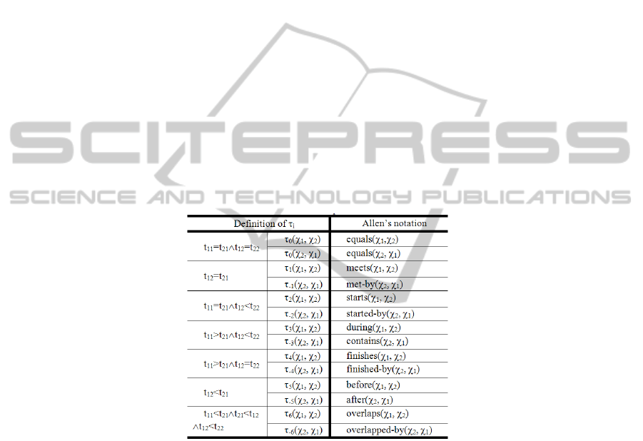
The definition of each τ
i
is provided with Table 1 implying the theorem T1, where
the durations of χ
1
and χ
2
are [t
11
, t
12
] and [t
21
, t
22
], respectively. This table shows the
complete list of temporal relations between two intervals, where 13 types of relations
are discriminated by the suffix ‘i’ (-6≤ i ≤6). This is in accordance with the conven-
tional notation [1, 9-13] which, to be strict, is for ‘temporal conjunctions (=∧
i
)’ but
not for pure ‘temporal relations (=τ
i
)’.
D1. χ
1
Κ
i
χ
2
⇔ (χ
1
Κ χ
2
) ∧ τ
i
(χ
1
, χ
2
)
T1. τ
-i
(χ
2
, χ
1
) ≡ τ
i
(χ
1
, χ
2
) (∀i∈{0,±1,±2,±3,±4,±5, ±6})
(Proof) Trivial in Table1. [Q.E.D.]
Table 1. List of temporal relations.
As easily understood, the properties of a TLC depend on those of the purely logi-
cal connective (
Κ ) and the temporal relations (τ
i
) involved. By the way, there are a
considerable number of trivial theorems concerning temporal relations such as (6)-
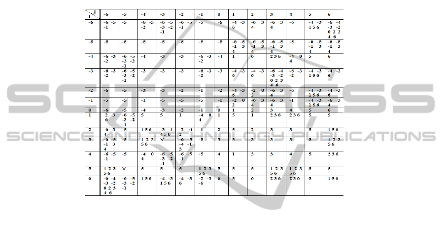
(13) below. All the possible cases of transitivity between two temporal relations are
listed up in Table 2. This table shows that the transitivity is not always determined
uniquely as easily calculated.
τ
i
(χ
1
,χ
2
)∧τ
0
(χ
2
,χ
3
) .⊃. τ
i
(χ
1
,χ
3
) .
(6)
τ
1
(χ
1
,χ
2
)∧τ
1
(χ
2
,χ
3
) .⊃. τ
5
(χ
1
,χ
3
) .
(7)
τ
1
(χ
1
,χ
2
)∧τ
3
(χ
2
,χ
3
) .⊃. τ
5
(χ
1
,χ
3
) .
(8)
τ
1
(χ
1
,χ
2
)∧τ
4
(χ
2
,χ
3
) .⊃. τ
5
(χ
1
,χ
3
) .
(9)
87

τ
1
(χ
1
,χ
2
)∧τ
5
(χ
2
,χ
3
) .⊃. τ
5
(χ
1
,χ
3
) .
(10)
τ
1
(χ
1
,χ
2
)∧τ
6
(χ
2
,χ
3
) .⊃. τ
5
(χ
1
,χ
3
) .
(11)
τ
2
(χ
1
,χ
2
)∧τ
1
(χ
2
,χ
3
) .⊃. τ
5
(χ
1
,χ
3
) .
(12)
τ
5
(χ
1
,χ
2
)∧τ
1
(χ
2
,χ
3
) .⊃. τ
5
(χ
1
,χ
3
) .
(13)
Table 2. List of all possible values of ‘k’ when τ
i
(P
1
,P
2
) ∧ τ
j
(P
2
,P
3
) .⊃. τ
k
(P
1
,P
3
) ( ‘∀’ denotes
that k=0,±1,±2,±3,±4,±5, ±6).
In order for explicit indication of absolute time elapsing, ‘Empty Event’ denoted
by ‘ε’ is introduced as D2 with the attribute ‘Time Point (A
34
)’ and the Standard of
absolute time ‘T
a
’. Usually people can know only a certain relative time point by a
clock that is seldom exact and that is to be denoted by another Standard in L
md
[8, 14].
Hereafter,
Δ denotes the total set of absolute time intervals. According to this scheme,
the suppressed absolute time-interval [t
a
, t
b
] of a locus χ can be indicated as (14).
D2. ε([t
i
,t
j
])⇔(∃x,y,g)L(x,y,t
i
,t
j
,A
34
,g,T
a
),
where [t
i
, t
j
]∈Δ (={[t
1
, t
2
] | t
1
<t
2
(t
1
, t
2
∈R)}).
χΠε([t
a
,t
b
]) .
(14)
A locus corresponding directly to the live image of a specific phenomenon outside is
called ‘Perceptual Locus’ and can be formulated with atomic locus formulas and
temporal conjunctions such as SAND (
∧
0
or Π) and CAND (∧
1
or •). This is not nec-
essarily the case for the other type of locus, so called, ‘Conceptual Locus’ that does
not correspond directly to such a live image but to such a generalized mental image or
knowledge piece as is conventionally represented by (2) with logical connectives
other than conjunctions also involved. This is essentially due to no interpreting a
negated atomic locus formula as a locus with a unique time-interval. That is, D1 is
exclusively for perceptual loci so far as it is. Whereas, such a theorem as
‘A⊃B.≡.~A∨B’ in standard logic can give us a good reason for the identity of a locus
88

formula with its negative in absolute time-interval, that is, negation-freeness of abso-
lute time passing under a locus referred to by its suppressed absolute time-interval.
Therefore, in order to make D1 valid also for conceptual loci, we introduce a meta-
function δ defined by D3 and its related postulates P1 and P2 as follows, where δ is
to extract the suppressed absolute interval of a locus formula
χ .
D3. δ(
χ )∈ Δ
P1. δ(~
α )=δ( α ), where α is an atomic locus formula.
P2. δ(χ)=[t
min
, t
max
], where t
min
and t
max
are respectively the minimum and the maxi-
mum time-point included in the absolute time-intervals of the atomic locus formulas,
either positive or negative, within χ.
These postulates lead to T2 (Theorem of negation-freeness of a suppressed absolute
time-interval) below.
T2. δ(~
χ )=δ( χ )
(Proof) According to P1 and P2, the time-interval of each atomic locus formula in-
volved in ~
χ is negation-free and therefore so are t
min
and t
max
in δ(~χ). [Q.E.D.]
The counterpart of the contrapositive in standard logic (i.e., A⊃B.≡.~B⊃~A) is
given as T3 (Tempo-logical Contrapositive) whose rough proof is as follows immedi-
ately below, where the left hand of ‘:’ refers to the postulates or theorems (e.g., PL is
a subset of those in pure predicate logic) employed at the process indicated by the
conventional meta-symbol ‘↔’ for bidirectional deduction.
T3. χ
1
⊃
i
χ
2
.≡.~χ
2
⊃
-i
~χ
1
(Proof)
D1: χ
1
⊃
i
χ
2
↔ (χ
1
⊃χ
2
)∧τ
i
(χ
1
,χ
2
)
PL: ↔ (~χ
2
⊃~χ
1
)∧τ
i
(χ
1
,χ
2
)
T2: ↔ (~χ
2
⊃~χ
1
)∧τ
i
(~χ
1
,~χ
2
)
D1: ↔ (~χ
2
⊃~χ
1
)∧τ
-i
(~χ
2
,~χ
1
)
D1: ↔ ~χ
2
⊃
-i
~χ
1
[Q.E.D.]
By the way, an empty event can be generated by T4, whose proof is trivial.
T4. χ.≡
0
.χ Πε(δ( χ ))
3 Knowledge Representation with TLCs
Perceptual loci are inevitably articulated by tempo-logical conjunctions. For example,
(3) or (4) is represented as (15).
A∧
5
B (≡ B∧
-5
A) .
(15)
As easily understood, any pair of loci temporally related in certain attribute spaces
can be formulated as (16)-(20) in exclusive use of SANDs, CANDs and empty
events.
χ
1
∧
2
χ
2
.≡. (χ
1
•ε)Πχ
2
.
(16)
89

χ
1
∧
3
χ
2
.≡. (ε
1
•χ
1
•ε
2
)Πχ
2
.
(17)
χ
1
∧
4
χ
2
.≡. (ε•χ
1
)Πχ
2
.
(18)
χ
1
∧
5
χ
2
.≡. χ
1
•ε•χ
2
.
(19)
χ
1
∧
6
χ
2
.≡. (χ
1
•ε
3
)Π(ε
1
•χ
2
)Π(ε
1
•ε
2
•ε
3
) .
(20)
Consider such somewhat complicated sentences as S4 and S5. The underlined parts
are deemed to refer to some events neglected in time and in space, respectively. These
events correspond with skipping of FAOs and are called ‘Temporal Empty Event’
and ‘Spatial Empty Event’, denoted by
ε
t
and ε
s
as empty events with g=G
t
and g=G
s
at D2, respectively. The images evoked by S4 and S5 can be formalized as (21) and
(22) in L
md
, respectively. A
15
and A
17
represent the attributes ‘Trajectory’ and ‘Mile-
age’, respectively, whose vales are relative to certain Standards (Refer to [8] for the
details).
(S4) The bus runs 10km straight east from A to B, and after a while, at C it meets the
street with the sidewalk.
(∃x
1
,x,y,z,p,q,k,k
1
,k
2
,k
3
)(L(x
1
,x,A,B,A
12
,G
t
,k)Π
L(x
1
,x,0,10km,A
17
,G
t
,k
1
)ΠL(x
1
,x,Point,Line,A
15
,G
t
,k
2
)
ΠL(x
1
,x,East,East,A
13
,G
t
,k
3
))•ε
t
•(L(x
1
,x,p,C,A
12
,G
t
,k)
ΠL(x
1
,y,q,C,A
12
,G
s
,k)ΠL(x
1
,z,y,y,A
12
,G
s
,k))
∧bus(x)∧street(y)∧sidewalk(z)∧p≠q .
(21)
(S5) The road runs 10km straight east from A to B, and after a while, at C it meets
the street with the sidewalk.
(∃x
1
,x,y,z,p,q,k,k
1
,k
2
)(L(x
1
,x,A,B,A
12
,G
s
,k)Π
L(x
1
,x,0,10km,A
17
,G
s
,k
1
)ΠL(x
1
,x,Point,Line,A
15
,G
s
,k
2
)
ΠL(x
1
,x,East,East,A
13
,G
s
,k
3
))•ε
s
•(L(x
1
,x,p,C,A
12
,G
s
,k)
ΠL(x
1
,y,q,C,A
12
,G
s
,k)ΠL(x
1
,z,y,y,A
12
,G
s
,k))
∧road(x)∧street(y)∧sidewalk(z)∧p≠q .
(22)
From the viewpoint of cross-media reference, the formula (22) can refer to such a
spatial event depicted as the still picture in Fig.1 while (21) can be interpreted into a
motion picture.
Fig. 1. Pictorial interpretation of the formula (22).
On the other hand, the causality represented by (2) can be formulated as (23) by
employing the temporal implication ‘⊃
5
’ or as its equivalent (24) with ‘⊃
-5
’. As easily
understood, these formulas are equivalent to such ones using temporal disjunctions as
parenthesized. By the way, (24) can be verbalized as S6.
B.⊃
-5
.A(≡~B∨
-5
A) .
(23)
90

~A.⊃
5
.~B (≡A∨
5
~B) .
(24)
(S6) Unless it gets cloudy, it does not rain later.
Without proper treatment of temporal relations, especially in Japanese [7], such a
somewhat quire contrapositive S8 would be yielded from S7.
(S7) The student does not study unless he is scolded.
(S8) The student is scolded if he studies.
Tempo-logical conjunctions are also applied to formulating event patterns involved in
such verb concepts as ‘carry’, ‘return’ and ‘fetch’ [8, 14] and temporal implications
are often employed for formalizing miscellaneous tempo-logical relations between
event concepts as knowledge pieces without explicit indication of time-intervals. For
example, an event ‘fetch(x,y)’ is necessarily finished by an event ‘carry(x,y)’ [8, 14].
This fact can be formulated as (25), which is not an axiom but a theorem deducible
from the definitions of event concepts here. Similarly, the tempo-logical relation
between ‘fetch(x,y)’ and ‘return(x)’ can be theorematized as (26). Furthermore, if
necessary, these can be temporally quantified as (27) and (28), respectively, where d
1
,
d
2
∈ Δ .
(∀x,y)fetch(x,y) .⊃
-4
. carry(x,y) . (25)
(∀x,y)fetch(x,y) .⊃
0
. return(x) . (26)
(∀x,y) (∀d
1
) (∃d
2
) fetch(x,y)Πε(d
1
) .⊃
-4
. carry(x,y)Πε(d
2
) . (27)
(∀x,y) (∀d
1
) (∃d
2
) fetch(x,y)Πε(d
1
) .⊃
0
. return(x)Πε(d
2
) . (28)
The postulate of reversibility of spatial events (PRS) [8] can be formulated as P1
using ‘≡
0
’, where χ and χ
R
is a perceptual locus and its ‘reversal’ for a certain spatial
event, respectively. These loci are substitutable with each other because of the prop-
erty of ‘≡
0
’.
P1. χ
R
.≡
0.
χ
The recursive operations to transform χ into χ
R
are defined by D4, where the reversed
values p
R
and q
R
depend on the properties of the attribute values p and q. For example,
at (22), p
R
=p, q
R
=q for A
12
; p
R
=-p, q
R
=-q for A
13
.
D4. (χ
1
•χ
2
)
R
⇔χ
2
R
•χ
1
R
(χ
1
Πχ
2
)
R
⇔ χ
1
R
Πχ
2
R
(L(x,y,p,q,a,G
s
,k))
R
⇔ L(x,y,q
R
,p
R
,a,G
s
,k)
By employing D4, (22) is transformed into (29) as its reversal and equivalent in PRS
to be verbalized as S9. That is, PRS is very helpful for paraphrasing of spatial events
variously expressed.
(∃x
1
,x,y,z,p,q,k,k
1
,k
2
,k
3
)(L(x
1
,x,C,p,A
12
,G
s
,k)Π
L(x
1
,y,C,q,A
12
,G
s
,k)ΠL(x
1
,z,y,y,A
12
,G
s
,k))
•ε
s
•(L(x
1
,x,B,A,A
12
,G
s
,k)ΠL(x
1
,x,0,10km,A
17
,G
s
,k
1
)
ΠL(x
1
,x,Point,Line,A
15
,G
s
,k
2
)
ΠL(x
1
,x,West,West,A
13
,G
s
,k
3
))
∧road(x)∧street(y)∧sidewalk(z)∧p≠q .
(29)
91

(S9)The road separates at C from the street with the sidewalk and, after a while, runs
10km straight west from B to A.
4 Tempo-logical Deduction with TLCs
Here is focused on tempo-logical syllogism as is formalized by (30), where logical
and temporal relations are calculated simultaneously in context of multiple tempo-
logical implications.
P
1
⊃
i
P
2
, P
2
⊃
j
P
3
|- P
1
⊃
k
P
3
,
where τ
i
(P
1
,P
2
) ∧ τ
j
(P
2
,P
3
) .⊃. τ
k
(P
1
,P
3
) .
(30)
The value of ‘k’ above is determined by the ordered pair (i,j) as shown in Table 2 and
the proof of such a proposition as (30) is given by a set of deductions formulated as
(31). The proof of such a formula as (31) is given by a set of deductions denoted as
(32) with the conventional symbol of deduction ‘→’ furnished with temporal rela-
tions.
P ⊃
n
Q .
(31)
X →
i (j )
Y, where τ
i
(X,Y) and τ
j
(P,Y), and j=n when Y=Q.
(32)
For example, consider the propositions A-F below and we can understand that F can
be deduced from D and E.
A=‘Tom studies’
B=‘Tom is scolded’
C=‘Tom is given candies’
D=‘Tom does not study unless he is scolded in advance’
E=‘Tom studies immediately before he is given candies’
F= ‘Tom is not given candies unless he is scolded in advance’,
where D, E and F are formulated as (33)-(35), respectively.
D .≡. ~B ⊃
5
~A .
(33)
E .≡. C ⊃
-1
A .
(34)
F .≡. ~B ⊃
5
~C .
(35)
The proof is as follows.
(Proof)
E, T3 :
~A⊃
1
~C .
(C1)
D :
~B→
5
(
5
)
~A .
C1, Table 2 :
→
1
(
5
)
~C (See Table2 at (i,j)=(5,1)) .
∴~B⊃
5
~C . [Q.E.D]
92

5 Application to Natural Language Understanding
The intelligent system IMAGES-M [8] can perform text understanding based on word
meaning descriptions as follows. Firstly, a text is parsed into a surface dependency
structure (or more than one if syntactically ambiguous). Secondly, each surface de-
pendency structure is translated into a conceptual structure (or more than one if se-
mantically ambiguous) using word meaning descriptions. Finally, each conceptual
structure is semantically evaluated.
The fundamental semantic computations on a text are to detect semantic anoma-
lies, ambiguities and paraphrase relations.
Semantic anomaly detection is very important to cut off meaningless computa-
tions. Consider such a conceptual structure as (36), where ‘A
39
’ is the attribute ‘Vital-
ity’. This locus formula can correspond to the English sentence ‘The desk is alive’,
which is usually semantically anomalous because a ‘desk’ does never have vitality in
the real world projected into the attribute spaces.
(∃x,y,k)L(y,x,Alive,Alive,A
39
,G
t
,k)∧desk(x) .
(36)
This kind of semantic anomaly can be detected in the following process.
Firstly, assume the concept of ‘desk’ as (37), where ‘A
29
’ refers to the attribute
‘Taste’. The special symbols ‘*’ and ‘/’ are defined as (38) and (39) representing
‘always’ and ‘no value’, respectively.
(λx)desk(x) ⇔ (λx)(…L*(y
1
,x,/,/,A
29
,G
t
,k
1
)∧…
∧ L*(y
n
,x,/,/,A
39
,G
t
,k
n
) ∧ …) .
(37)
X* ⇔ (∀d∈Δ)X Π ε(d) .
(38)
L(…,/,…) ⇔ ~(∃p) L(…,p,…) .
(39)
Secondly, the postulates (40) and (41) are utilized. The formula (40) means that if one
of two loci exists every time interval, then they can coexist. The formula (41) states
that a matter never has different values of an attribute with a standard at a time.
X ∧ Y* .⊃. X Π Y .
(40)
(∀x,y,z, p
1
,q
1
, p
2
,q
2
,a,g,k) L(x,y,p
1
,q
1
,a,g,k)ΠL(z,y,p
2
,q
2
,a,g,k)
.⊃. p
1
=p
2
∧ q
1
=q
2
.
(41)
Lastly, the semantic anomaly of ‘alive desk’ is detected by using (36)-(41). That is,
the formula (42) below is finally deduced from (36)-(40) and violates the com-
monsense given by (41), that is, “ Alive ≠ / ”.
(∃x,y,z,k
1
,k
2
)L(y,x,Alive,Alive,A
39
,G
t
,k
1
)Π L(z,x,/,/,A
39
,G
t
,k
2
) .
(42)
This 15 at the insect on the desk, which is still alive.
If a text has multiple plausible interpretations, it is semantically ambiguous. For
example, S11 alone has two plausible interpretations (43) and (44) different at the
underlined parts, implying ‘Tom with the stick’ and ‘Jim with the stick’, respectively.
(S11) Jim follows Tom with the stick.
(∃x,k)(L(Tom,Tom,p,q,A
12
,G
t
,k)
ΠL(Tom,x,Tom,Tom,A
12
,G
t
,k))• L(Jim,Jim,p,q,A
12
,G
t
,k)∧p≠q ∧stick(x) .
(43)
93

(∃x,k)L(Tom,Tom,p,q,A
12
,G
t
,k)•(L(Jim,Jim,p,q,A
12
,G
t
,k) Π
L(Jim,x,Jim,Jim,A
12
,G
t
,k))∧p≠q ∧stick(x) .
(44)
Among the fundamental semantic computations, detection of paraphrase relations is
the most essential because it is for detecting equalities in semantic descriptions and
the other two are for detecting inequalities in them. In our system, if two different
texts are interpreted into the same locus formula, they are paraphrases of each other.
The understanding process above is completely reversible except that multiple
paraphrases can be generated by tempo-logical reasoning as shown in Fig.2-a because
event patterns are sharable among multiple word concepts. Fig.2-b shows the graph-
ical interpretation of the kernel structure of the input sentence, namely, “with stick
Tom precedes Jim”, whose formulation in L
md
is the same as (43) (Refer to [8] for the
details).
(Input)
With the long red stick Tom precedes Jim.
(Output)
Tom with the long red stick goes before Jim goes.
Jim goes after Tom goes with the long red stick.
Jim follows Tom with the long red stick.
Tom carries the long red stick before Jim goes.
The stick moves simultaneously when Tom goes.
………………….
t1 t2 t3 Time
p
Tom
A12
Jim
q
stick
t1 t2 t3 Time
p
Tom
A12
Jim
q
stick
(a) (b)
Fig. 2. (a) Text paraphrasing by tempo-logical reasoning, and (b) Graphical interpretation of
“with stick Tom precedes Jim”.
6 Conclusions
The theory of tempo-logical connectives introduced in MIDST was extended so as to
be applicable to intuitive spatiotemporal knowledge expressed in natural language in
order to facilitate intuitive human-robot interaction much better. This extension was
concentrated on providing the theory with tempo-logical connectives other than tem-
po-logical conjunctions, where the principal definitions and postulates have been
induced from several psycholinguistic experiments [7]. To remark reversely, they
have been already psycho-linguistically validated.
MIDST is intended to provide a formal system represented in L
md
for natural or
intuitive semantics of spatiotemporal language [14]. This formal system is one kind of
applied predicate logic consisting of axioms and postulates subject to human percep-
tion of space and time while the other similar systems in Artificial Intelligence [1-6,
9-13] are intended to be objective, namely, independent of human perception process
and do not necessarily keep tight correspondences with natural language. For exam-
ple, the postulates P1 and P2 of human perception of time and TLCs have brought the
tempo-logical contrapositive, which leads to the naturalness of tempo-logical syllo-
gism without explicit indication of time points. Furthermore, such paraphrasing based
on spatiotemporal reasoning as in Fig.2-a shows that explicit description of word
concepts grounded in loci in attribute spaces can simulate mental image processing in
humans well enough for text-picture cross-reference both in spatial and temporal
94

extents [8], which is very essential for ordinary people to have intuitive access to
intelligent multimedia systems. Our future work will include further explication of
potential expressiveness of TLCs.
This work is partially funded by Japanese Gov., MEXT (Grant No.23500195).
References
1. Allen, J. F.: Towards a general theory of action and time, Artificial Intelligence, Vol.23-2
(1984) 123-154.
2. Beek, P.: Reasoning about qualitative temporal information. Artificial Intelligence, Vol.58
(1992) 297-326.
3. Haddaw, P. A.: Logic of time, chance, and action for representing plans, Artificial Intelli-
gence, 80-2 (1996) 243-308.
4. McDermott, D. V.: A temporal logic for reasoning about processes and plans, Cognitive
Science, 6 (1982) 101-155.
5. Shoham, Y.: Time for actions: on the relationship between time, knowledge, and action,
Proc. of IJCAI 89, Detroit, MI (1989) 954-959.
6. Egenhofer, M., Khaled, K.: Reasoning about Gradual Changes of Topological Relations,
Proc. of International Conference GIS—From Space to Territory: Theories and Methods of
Spatio-Temporal Reasoning, Pisa, Italy (1992) 196-219.
7. Yokota, M.: A psychological experiment on human understanding process of natural lan-
guage (in Japanese), Trans. of IEICE Japan, 71-D-10 (1988) 2120-2127.
8. Yokota, M.: An approach to natural language understanding based on a mental image
model, Proc. of the 2
nd
NLUCS (2005) 22-31.
9. Freksa, C.: Temporal reasoning based on semi-intervals. Artificial Intelligence, 54 (1992)
199-227.
10. Jungclaus, R., Saake, G., Hartmann, T., Sernadas, C.: TROLL- A Language for Object-
Oriented Specification of Information Systems, ACM Transactions on Information Sys-
tems, 14(2) (1996) 175-211.
11. Bruce, B. C.: A Model for Temporal References and Its Application in a Question Answer-
ing Program, Artificial Intelligence, 3 (1972) 1-25.
12. Torsun, I. S.: Foundations of Intelligent Knowledge-Based Systems, Academic Press
(1995).
13. Abadi, M., Manna, Z.: Nonclausal Deduction in First-Order Temporal Logic, Journal of the
Association for Computing Machinery, 37-2 (1990) 279-317.
14. Yokota, M.: Systematic Formulation and Computation of Subjective Spatiotemporal
Knowledge Based on Mental Image Directed Semantic Theory, Proc. of the 6
th
NLPCS
(2009) 133-143.
95