
A Binary Neural Network Framework for Attribute Selection and
Prediction
Victoria J. Hodge, Tom Jackson and Jim Austin
Department of Computer Science, University of York, York, U.K.
Keywords: Attribute Selection, Feature Selection, Binary Neural Network, Prediction, k-Nearest Neighbour.
Abstract: In this paper, we introduce an implementation of the attribute selection algorithm, Correlation-based Feature
Selection (CFS) integrated with our k-nearest neighbour (k-NN) framework. Binary neural networks
underpin our k-NN and allow us to create a unified framework for attribute selection, prediction and
classification. We apply the framework to a real world application of predicting bus journey times from
traffic sensor data and show how attribute selection can both speed our k-NN and increase the prediction
accuracy by removing noise and redundant attributes from the data.
1 INTRODUCTION
Prediction is the assumption that the future trend of
variations in the value of a time-series variable will
mirror the trend of variations in the value of the
same variable for similar historical time-series.
There is a wide variety of prediction algorithms
including: ARCH (Engle, 1982), ARIMA (Box and
Jenkins, 1970), neural networks (Bishop, 1995) and
support vector machine regression (Brucker et al.,
1997). The prediction algorithms typically have two
phases of operation: a training phase where the
algorithm learns a representation of the data and a
prediction phase where the algorithm generates
predictions for new records using the learned model.
For prediction, the quality of the input data is
critical; redundant and irrelevant attributes can slow
execution and reduce accuracy. Redundant attributes
also push the data to the tails of the distribution as
the higher dimensionality spreads the data’s convex
hull. Attribute selectors reduce the dimensionality of
data by selecting a subset of attributes (Kohavi and
John, 1997). They remove irrelevant and redundant
information, reduce the size of the data and clean it.
This allows machine-learning algorithms such as
predictors to operate more effectively.
There is a wide variety of attribute selection
including: Correlation-based Feature Selection (Hall,
1998); Information Gain (Quinlan, 1986); Chi-
square Selection (Liu and Setiono, 1996); and,
Support Vector Machines Selection (Guyon et al.,
2002). There are two approaches for attribute
selection (Kohavi and John, 1997). Filters are
independent of the actual algorithm and tend to be
simple, fast and scalable. Wrappers use the
algorithm to select attributes. Wrappers can produce
better performance than filters as the attribute
selection process is optimised for the particular
algorithm. However, they can be computationally
expensive for high dimensional data as they must
evaluate many candidate sets using the classifier.
Attribute selection is often used in conjunction
with data mining algorithms such as k-NN. K-NN is
a widely used algorithm (Cover and Hart, 1967);
(Hodge, 2011) that examines vector distances to
determine the nearest neighbours. However,
standard k-NN is computationally slow for large
datasets. We have previously developed a binary
neural network-based k-NN (Hodge and Austin,
2005) using the Advanced Uncertain Reasoning
Architecture (AURA) framework. It is efficient and
scalable, being up to four times faster than the
standard k-NN (Hodge et al., 2004). We extended
AURA k-NN to prediction in Hodge et al., (2011).
The main contribution of this paper is to:
introduce the CFS attribute selector into the AURA
k-NN framework and demonstrate the attribute
selector’s utility for prediction on a real world
problem. Using attribute selection with prediction to
reduce the data size will further speed processing.
510
J. Hodge V., Jackson T. and Austin J..
A Binary Neural Network Framework for Attribute Selection and Prediction.
DOI: 10.5220/0004150705100515
In Proceedings of the 4th International Joint Conference on Computational Intelligence (NCTA-2012), pages 510-515
ISBN: 978-989-8565-33-4
Copyright
c
2012 SCITEPRESS (Science and Technology Publications, Lda.)

2 AURA
AURA (Austin, 1995) is a set of methods for pattern
recognition. AURA is ideal to use as the basis of an
efficient k-NN predictor as it is able to partial match
during retrieval so it can rapidly find records that are
similar to the input – the nearest neighbours. It has
a number of advantages over standard neural
networks including rapid one-pass training, high
levels of data compression, network transparency
and a scalable architecture. These are enhanced with
our robust data encoding method to map numeric
attributes onto binary vectors for training and recall.
2.1 Time-series
To estimate bus journey times, the system must
incorporate a time component. In this paper, the
vectors represent time-series of spatially-distributed
sets of traffic sensors. To produce the time-series
vector X
j
, we buffer each sensor’s readings for a
preset time interval PT and concatenate the buffers
to form the time series X
j
TS
. Buffering always
preserves the temporal ordering of the data. X
j
TS
is
{
x
1t-2
, x
1t-1
, x
1t
, x
2t-2
, … ,x
yt-2
, x
yt-1
, x
yt
} for PT of three
time slices {t-2, t-1, t} and y sensors.
2.2 Learning
AURA uses binary input I and output O vectors to
store records in a CMM, M as in fig. 1. First, any
numeric attributes must be quantised (binned) as the
data to be trained into the CMM is binary.
Quantisation maps a range of input values for
attribute a onto each bin. Each individual bin maps
to a unique integer. This identifies the bit to set in
the AURA input vector and a unique row in the
CMM (see Hodge and Austin (2005) for details).
Equi-width quantisation subdivides each attribute
into b equal width bins across its range of values.
The even widths of the bins ensures that the inter-bin
distances are all equivalent and that the quantised
data can be used to approximate the Euclidean
distance. Once the bins and integer mappings have
been determined, we map the records onto binary
vectors to train into the CMM during learning. Each
binary vector represents a pattern from the data set.
For an attribute with five bins, the five binary
representations are then bin
0
= 00001, bin
1
= 00010,
bin
2
= 00100 etc. The bins corresponding to the data
values in X
j
TS
are set to 1 and all other bins are set to
0. The binary representations for all attributes and
their respective time slices are concatenating to form
I
j
. Thus, I
j
is a learning pattern stored in the CMM to
allow the particular record to be stored and indexed.
The CMM, M, is initialised with all weights set
to 0. Training stores the binary patterns for all N
records in the data set in M. Each binary pattern I
j
is
associated with a unique identifier pattern O
j
. Each
O
j
has a single bit set to index a unique column in M
and to uniquely index I
j
. At each training step, any
matrix elements excited by both the input and output
patterns are set to 1. This process is given in eq. 1.
)(
T
jjj
OIM
where is logical OR
(1)
2.3 Recall
AURA recall is the dot product of a recall input
vector R
k
and M. R
k
may be either a binary vector or
an integer vector. For prediction, we use an integer
vector to allow us to emulate Euclidean distance. For
attribute selection (described later), we use a binary
vector to count attribute values and co-occurrences.
For prediction, the integer recall vector R
k
is
generated for each new query using a set of
concatenated parabolic kernels. The kernels
represent scores which decrease in value with the
distance from the query value and emulate Euclidean
distance (see (Hodge and Austin, 2005) for details).
Each kernel is centred on the bin representing each
attribute value for the query record so that bin
receives the highest score (the dotted values in Fig.
1). The best matching historical records will receive
the highest scores. R
k
is applied to M to retrieve the k
best matches and the values in R
k
multiply the rows
of the matrix as in eq.2 and Fig. 1. The columns of
M are summed according to the values on the rows
indexed by R
k
multiplied by the CMM weights to
produce a summed output vector S
k
as given in eq. 2.
M
k
R
T
k
S
(2)
In Fig. 1, rows 0 to 4
represent traffic sensor
Sensor
1
, the variable is vehicle flow and the time
slice within the time-series is t-2. For row 4,
columns 2 and 3 (indexing from 0 on the left) score
9 as the set bits in columns 2 and 3 align with the
score of 9 for row 4. In contrast, column 0 receives a
score of 0 as the set bit in column 0 aligns with row
0 which scores 0 from the recall pattern R
k
.
For partial matching, we use L-Max thresholding
which retrieves at least L top matches. It finds the L
highest values in the output vector S
k
and sets the
corresponding vector element to one in the binary
output vector T
k
. For AURA k-NN, L is set to the
value of k; the number of nearest neighbours.
ABinaryNeuralNetworkFrameworkforAttributeSelectionandPrediction
511
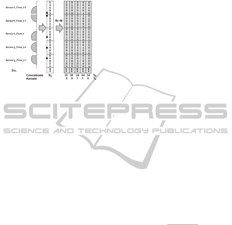
Figure 1: Diagram showing the application of kernels to a
CMM to find the nearest neighbours. The retrieval input
vector R
k
is produced by applying kernels. The dot is the
bin representing the query value for each attribute. AURA
multiplies R
k
*M, using the dot product, sums each column
to produce S
k
and thresholds S
k
to produce T
k
.
2.4 Prediction
We maintain a lookup table of values for the
prediction attribute t+n time steps ahead for each
historical record. After recall, AURA k-NN cross-
references the historical records from the set of
column indices in T
k
, sums the t+n attribute values
for these matching columns and calculates the mean
value for the prediction attribute n time steps ahead.
3 ATTRIBUTE SELECTION
In Hodge et al., (2006), we developed two attribute
selection approaches in AURA: univariate Mutual
Information (MI) and multivariate Probabilistic Las
Vegas. MI selected the attributes up to 100 times
faster when implemented using AURA compared to
a standard technique. Here we develop another
attribute selector in AURA. This will provide a
range of attribute selectors so that the most suitable
may be chosen for each application.
3.1 CFS Selection
Hall (1998) proposed the multivariate Correlation-
based Feature Subset Selection (CFS) which
measures the association strength between pairs of
attributes. The advantage of a multivariate filter such
as CFS compared to a univariate filter such as MI
lies in the fact that a univariate filter does not
account for attribute interactions. Hall and Smith
(1997) demonstrated that CFS chooses attribute
subsets that improve the accuracy of common
machine learning algorithms (including k-NN).
3.1.1 Quantisation
In AURA CFS, any numeric attributes (including
class attributes) are quantised to map the data to
AURA using Fayyad and Irani’s (1993) quantisation
method which aims to minimise the entropy, see
Hall (1998) for details.
3.1.2 Symmetrical Uncertainty
Hall and Smith (1997) use a revised information
gain measure to estimate the correlation between
discrete attributes. If a and b are discrete random
attributes, the entropy for all records in the training
data set for value i of attribute a is given by eq. 3:
ai
ipipaEnt ))((
2
log)()(
(3)
The data values of a can be partitioned according to
the values of the second attribute b. If the entropy of
a with respect to the partitions induced by b is less
than the entropy of a prior to partitioning then there
is a correlation (information gain) between attributes
a and b, this is given in eq. 4 and 5 where i and j are
attribute values of attributes a and b respectively.
ai
jipjip
bj
jpbaEnt ))|((
2
log)|()()|(
(4)
)|()(),( baEntaEntbaGain
(5)
Information Gain is biased toward attributes that
have a larger number of data values. Hence, Hall and
Smith (1997) use symmetrical uncertainty (SU) to
replace information gain as given by eq. 6.
)()(
),(
0.2),(
bEntaEnt
baGain
baSU
(6)
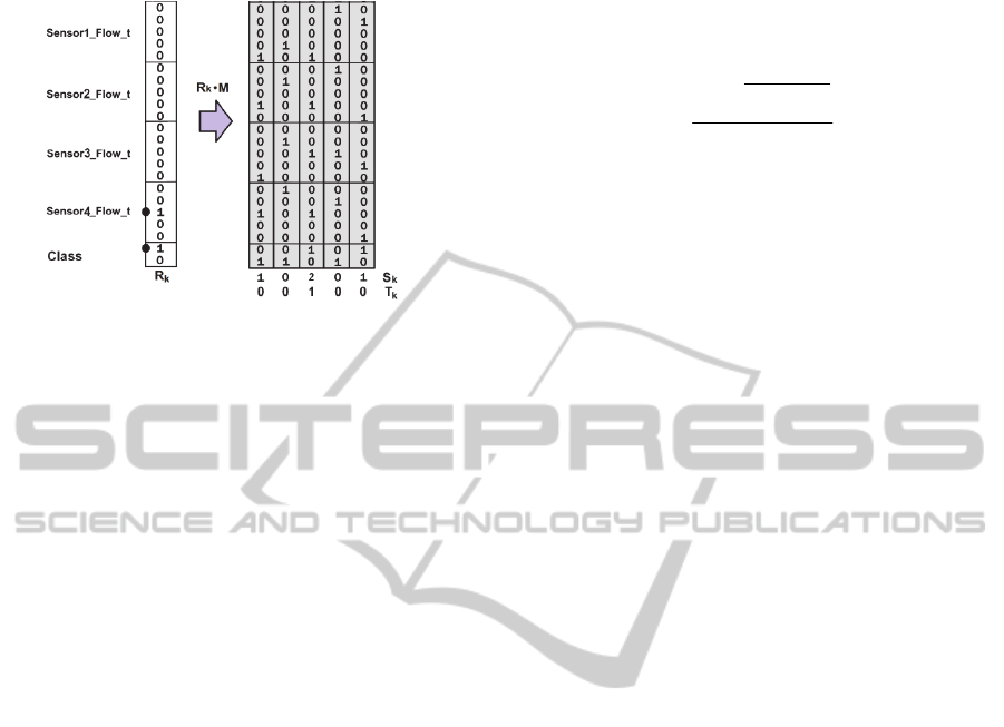
3.2 Mapping CFS to AURA
For attribute selection, the class values are also
trained into the CMM as extra rows; the class is
treated as an extra attribute as shown in Fig. 2.
AURA is used to calculate Ent(a), Ent(b) and
Gain(a,b). Ent(a) is based on the calculation of the
total count of data records for a particular attribute
value a
i
. AURA excites the row in the CMM
corresponding to a
i
which produces a summed
output vector as described in eq. 2 with a one for
every record that has value a
i
. The total count is the
count of the number of ones in T
k
in Fig. 2. Ent(b) in
eq. 6 calculates the total count of data records for a
IJCCI2012-InternationalJointConferenceonComputationalIntelligence
512
particular attribute value b
j
as per a
i
.
Figure 2: Diagram showing the use of the CMM for
attribute selection. The class attribute is included. The
retrieval input vector R
k
is binary for attribute selection
whereas Fig. 2 has an integer retrieval vector. The dot is
the value for each attribute (a quantisation bin).
Gain(a, b) is based on the calculation of Ent(a)
and Ent(a|b). Ent(a|b) counts the number of co-
occurrences of a
i
with b
j
. AURA excites both CMM
rows corresponding to a
i
and b
j
as in Fig. 2. S
k
has a
two in the column of every record with a co-
occurrence of a
i
with b
j
. By thresholding S
k
at 2, we
find all co-occurrences. The total co-occurrence
count is the count of the number of ones in T
k
.
3.3 Selecting the Attribute Subset
CFS uses Best First Forward Search (Hall, 1998) to
search the attribute space, greedily adding individual
attributes to the chosen subset. Search terminates
when five consecutive fully expanded subsets show
no improvement over the current best subset.
4 JOURNEY TIME ESTIMATION
We analyse our prediction framework to see if it
could form part of a system to analyse mean bus
journey times in York, UK. This system would
provide an estimate of the level of congestion
encountered by buses so other vehicles can be routed
to less congested roads We plan to estimate the bus
journey times using other traffic sensor data to plug
the gaps when actual bus data is not available.
To combine different bus routes along a road into
an overall congestion estimate, we use journey time
ratio. For buses, the bus journey time ratio is the
journey time for a particular bus travelling the route
between a particular pair of bus stops divided by the
90
th
percentile historical journey time for that route.
Mean journey time ratio is defined as the mean ratio
across all buses travelling all routes along the road in
a particular time period p as given by eq. 7.
N
bjt
bjt
p
mean
N
nr
yxr
yxr
1
90
R
1
),:(
),:(
(7)
Where bjt
(r:,x,y)
is the bus journey time for route r
between stops x and y; bjt
(r:x,y)
90
is the 90
th
percentile
historical bus journey time for route r between stops
x and y and N is the number of buses during the time
period. Mean
p
will be <1 if the road is uncongested
and ≥ 1 if the road is congested as bus journey times
will exceed the 90
th
percentile journey times.
The sensors on the roads in York output vehicle
flow (the number of vehicles passing over the sensor
during a specific time period). The sensor data forms
a pattern of the current traffic conditions for a time
period p which we associate with the bus journey
time ratio mean
p
for the same time period p
,
using
the data’s timestamps. AURA k-NN uses the sensor
patterns as the input vectors and predicts the
expected bus journey time ratio from the matching
sensor pattern associations.
5 EVALUATION
The data comprises traffic sensor and inbound bus
journey data from Fulford Road in York from
05/10/2010 to 28/03/2011. There are ten sensors
each generating a flow value every five minutes. We
use 12 time steps representing one hour’s duration as
our time series. There are five possible bus routes
along the road section under investigation. Bus
journeys are aggregated over five minute periods to
match the periodicity of the traffic sensors.
We only consider time periods when two or more
buses departed the final stop to smooth any
anomalous readings. The data have been cleaned by
removing erroneous bus journey times (80 seconds ≤
valid ≤ 2400 seconds). The data are still very noisy
but will allow a thorough test of the algorithms and
configurations under evaluation. The data set has
1932 records which we split 2/3 for training and 1/3
for testing giving 1288 training records and 644 test
records. We perform the attribute selection on
training data only. Each algorithm’s parameters were
optimised using only the training data: we evaluated
a similar number of parameter sets for each
algorithm for fairness. The test data was applied to
each learned model to get the prediction accuracy.
ABinaryNeuralNetworkFrameworkforAttributeSelectionandPrediction
513
We produced three data configurations: all
records in chronological order (DataSet1); all
records in alphabetical order of date/time
(DataSet2); and, all records in reverse alphabetical
order of date/time (DataSet3).
The evaluation compares the RMSE of a multi-
layer perceptron (MLP) used by Vlahogianni et al.
(2005), a support vector machine (SVM) used by
Labeeuw et al. (2009) and three configurations of
the AURA k-NN: no time-series data (AURA
nts
);
time-series length 12 (AURA
ts
) and time-series
length 12 but only the sensors selected by CFS
(AURA
CFSts
). For CFS, we split the class (mean
p
)
into two bins (as in Fig. 2), if mean
p
<1 then map to
bin
uncongested
otherwise map to bin
congested
.
Each algorithm was applied to the three data sets
using all attributes unless stated and a mean RMSE
was calculated across the three data sets. The results
are listed in table 1. In table 2, we compare the
RMSE of the algorithms using just the chronological
(true) order, DataSet1. Table 3 lists the parameter
settings for AURA k-NN using CFS across the three
data sets to demonstrate whether the variation in
parameters is needed. Table 4 lists the training times
on all of DataSet1 for AURA k-NN and AURA k-
NN learning only the attributes selected using CFS.
6 RESULTS
We examine the attributes selected and the
prediction accuracy of the various algorithms next.
6.1 Attribute Selection
For the three data sets, CFS selected:
DataSet1: Sensor3, Sensor6, Sensor9
DataSet2: Sensor1, Sensor2, Sensor3, Sensor6
DataSet3: Sensor3, Sensor6, Sensor9
CFS has reduced the data dimensionality from 10
sensors to 3 for two of the data configurations and
reduced the dimensionality to 4 for the other. This
will speed both training and prediction for k-NN.
The subsets for DataSet1 and DataSet3 are identical
and sensors 3 and 6 are present in all subsets
indicating some consistency. This data is noisy and
temporal data is likely to have trends. These will
affect the data when it is split into train and test sets
which may explain the differences in DataSet2. Next
we evaluate the prediction accuracy to ensure that
this dimensionality reduction has not compromised
the accuracy.
6.2 Prediction Accuracy
Table 1: Table comparing the mean RMSE (RMSEµ) for
the prediction algorithms over the three data sets. The
highest prediction accuracy is shown in bold.
Algorithm
MLP SVM AURA
nts
AURA
ts
AURA
CFSts
RMSEµ
0.1795 0.1722 0.1799 0.1750
0.1709
Table 2: Table comparing the mean RMSE (RMSEµ) for
the algorithms over the chronologically ordered DataSet1.
The highest prediction accuracy is shown in bold.
Algorithm
MLP SVM AURA
nts
AURA
ts
AURA
CFSts
RMSEµ
0.1826 0.1626 0.1695 0.1671
0.1603
Tables 1 and 2 show that CFS attribute selection
coupled with time-series data improves the
prediction accuracy of AURA k-NN. Thus, CFS has
both reduced the dimensionality and increased the
accuracy. Only the AURA k-NN using CFS attribute
selection is able to outperform the SVM benchmark.
6.3 Parameters
Table 3: Table listing the parameter settings for AURA
CFSts
across the three data sets. The three parameter variables
are the number of neighbours retrieved (k), the number of
quantisation bins and the range of values for quantisation.
Dataset
K value Bins Range
1
19 15 [0, 120]
2
24 15 [0, 120]
3
14 11 [0, 120]
Table 3 shows that across the three data sets the
AURA k-NN parameters require tuning to maximise
prediction accuracy. This variation also applied to
the parameters of both the MLP and SVM. It is
important that a prediction algorithm can perform
this optimisation quickly and efficiently. Using CFS
to reduce the data dimensionality will speed the
parameter optimisation further as shown in table 4.
Both standard MLPs and SVMs are slow to train as
they require multiple passes through the data. Zhou
et al. (1999) determined that the AURA k-NN trains
up to 450 times faster than an MLP.
6.4 Training Time
For AURA k-NN, the training time contributes the
bulk of the processing time whereas retrieving the
matches is much quicker (Hodge et al., 2004). Using
attribute selection prior to training reduces the
training time by almost half by reducing the data
size. Attribute selection is a one off cost whereas the
AURA CMM must be trained each time the system
is started so the key is minimising the training time.
IJCCI2012-InternationalJointConferenceonComputationalIntelligence
514

Table 4: Table comparing the mean training time for
AURA k-NN using time-series data compared to AURA
k-NN with CFS on the same data. The mean was
calculated over five runs.
AURA
ts
AURA
CFSts
Training time (secs)
0.30
0.17
7 CONCLUSIONS
In this paper, we have introduced a unified
framework for attribute selection and prediction.
Classification is also available in the framework
(Hodge and Austin, 2005); (Krishnan et al., 2010).
Previously, we demonstrated two attribute
selection approaches in AURA (Hodge et al., 2006).
We have now added the multivariate CFS selector
which is based on entropy. No attribute selector
excels on all data or all tasks so we need a range of
selectors to select the best for each task. We showed
that CFS improved the prediction accuracy of the
AURA k-NN on the real world task of bus journey
prediction. We demonstrated that using attribute
selection to reduce the dimensionality reduces the
training time allowing larger data to be processed.
The AURA framework described is flexible and
easily extended to other attribute selection
algorithms. Ultimately, we will provide a parallel
and distributed data mining framework for attribute
selection, classification and prediction drawing on
our previous work on parallel (Weeks et al., 2002)
and distributed AURA (Jackson et al., 2004).
REFERENCES
Austin, J., 1995. Distributed Associative Memories for
High Speed Symbolic Reasoning. In IJCAI: Working
Notes of Workshop on Connectionist-Symbolic
Integration, pp. 87-93.
Bishop, C., 1995. Neural networks for pattern recognition,
Oxford University Press, Oxford, UK.
Box, G., Jenkins, G., 1970. Time series analysis:
Forecasting and control, San Francisco: Holden-Day.
Cover T., Hart P, 1967. Nearest neighbor pattern
classification. IEEE Transactions on Information
Theory 13(1): 21–27.
Engle, R., 1982. Autoregressive Conditional
Heteroscedasticity with Estimates of the Variance of
UK Inflation. Econom., 50: 987-1008.
Fayyad, U., Irani K., 1993. Multi-Interval Discretization
of Continuous-Valued Attributes for Classification
Learning. In Procs International Joint Conference on
Artificial Intelligence, pp. 1022-1029.
Guyon, I. et al., 2002. Gene selection for cancer
classification using support vector machines. Mach.
Learn., 46(1): 389-422
Hall, M., 1998. Correlation-based Feature Subset
Selection for Machine Learning. Ph.D. Thesis,
University of Waikato, New Zealand.
Hall, M., Smith, L., 1997. Feature subset selection: a
correlation based filter approach. In, International
Conference on Neural Information Processing and
Intelligent Information Systems, pp. 855-858.
Hodge, V., 2011. Outlier and Anomaly Detection: A
Survey of Outlier and Anomaly Detection Methods.
LAMBERT Academic Publishing, ISBN: 978-3-8465-
4822-6.
Hodge, V., Austin, J., 2005. A Binary Neural k-Nearest
Neighbour Technique. Knowl. Inf. Syst. (KAIS), 8(3):
276-292, Springer-Verlag London Ltd.
Hodge, V. et al., 2004. A High Performance k-NN
Approach Using Binary Neural Networks. Neural
Netw., 17(3): 441-458, Elsevier Science.
Hodge, V. et al., 2006. A Binary Neural Decision Table
Classifier. NeuroComputing, 69(16-18): 1850-1859,
Elsevier Science.
Hodge, V. et al., 2011. Short-Term Traffic Prediction
Using a Binary Neural Network. 43rd Annual UTSG
Conference, Open University, UK, January 5-7.
Jackson, T. et al., 2004. Distributed Health Monitoring for
Aero-Engines on the Grid: DAME. In Procs of IEEE
Aerospace, Montana, USA, March 6-13.
Kohavi, R. John, G., 1997. Wrappers for Feature Subset
Selection. In Artif. Intell. J., Special Issue on
Relevance, 97(1-2): 273-324
Krishnan, R. et al., 2010. On Identifying Spatial Traffic
Patterns using Advanced Pattern Matching
Techniques. In Procs of Transportation Research
Board (TRB) 89th Annual Meeting, Washington, D.C.
Labeeuw, W. et al., 2009. Prediction of Congested Traffic
on the Critical Density Point Using Machine Learning
and Decentralised Collaborating Cameras.
Portuguese
Conference on Artificial Intelligence, pp. 15-26.
Liu, H., Setiono, R., 1995. Chi2: Feature selection and
discretization of numeric attributes. In Procs IEEE 7th
International Conference on Tools with Artificial
Intelligence, pp. 338-391.
Quinlan, J., 1986. Induction of Decision Trees. Mach,
Learn., 1: 81-106.
Vlahogianni, E. et al., 2005. Optimized and meta-
optimized neural networks for short-term traffic flow
prediction: A genetic approach, Transp. Res. Part C:
Emerging Technologies, 13(3) (2005): 211-234.
Weeks, M. et al., 2002. A Hardware Accelerated Novel IR
System. In Procs 10th Euromicro Workshop (PDP-
2002), Gran Canaria, Jan. 9–11, 2002.
Zhou, P. et al., 1999. High Performance k-NN Classifier
Using a Binary Correlation Matrix Memory. In Procs
Advances in Neural Information Processing Systems
Vol. II, MIT Press, Cambridge, MA, USA, 713-719.
ABinaryNeuralNetworkFrameworkforAttributeSelectionandPrediction
515
