Focused Image Color Quantization using Magnitude Sensitive

Competitive Learning Algorithm

Enrique Pelayo, David Buldain and Carlos Orrite

Aragon Institute for Engineering Research, University of Zaragoza, Zaragoza, Spain

Keywords:

Color, Quantization, Competitive Learning, Neural Networks, Saliency.

Abstract:

This paper introduces the Magnitude Sensitive Competitive Learning (MSCL) algorithm for Color Quanti-

zation. MSCL is a neural competitive learning algorithm, including a magnitude function as a factor of the

measure used for the neuron competition. This algorithm has the property of distributing color vector proto-

types in certain data-distribution zones according to an arbitrary magnitude locally calculated for every unit.

Therefore, it opens the possibility not only to distribute the codewords (colors of the palette) according to their

frequency, but also to do it in function of any other data-dependent magnitude focused on a given task. This

work shows some examples of focused Color Quantization where the objective is to represent with high detail

certain regions of interest in the image (salient area, center of the image, etc.). The oriented behavior of MSCL

permits to surpass other standard Color Quantization algorithms in these tasks.

1 INTRODUCTION

With the great development of the informatics in our

society, large amount of scanned documents and im-

ages are being transmitted and stored. Therefore,

some kind of image compression, to reduce the num-

ber of color patterns in the image, becomes neces-

sary to reduce storage and transmission resources.

This process is generally achieved by means of Vec-

tor Quantization (VQ) techniques. The idea behind

VQ is the selection of a reduced number of prototypes

that accurately represent the whole data set. When

each data sample is a vector representing the color

of a pixel, it is called Color Quantization (CQ). This

type of algorithms are being widely used in certain ap-

plications related to segmentation, compression, and

transmission of images.

A subset of VQ algorithms comprises Compet-

itive Learning (CL) methods, where a neural net-

work model is used to ﬁnd an approach of VQ cal-

culation in an unsupervised way. The main advan-

tage over other VQ algorithms is that CL is sim-

ple and easily parallelizable. Well known CL ap-

proaches are K-means (Lloyd, 1982), including some

of its variants as Weighted K-Means and improve-

ments (Celebi, 2011), Frequency Sensitive Compet-

itive Learning (FSCL) (Ahalt et al., 1990), Rival Pe-

nalized Controlled Competitive Learning (Xu et al.,

1993), the Self-Organizing Map (SOM) (Kohonen,

2001), the Neural Gas (NG) (Martinetz et al., 1993),

Elastic Net (EN) (Durbin and Willshaw, 1987) and

Generative Topographic Mapping (GTM) (Bishop

et al., 1998). Some of these methods, or variants,

have already been used in CQ and Color Segmen-

tation tasks. Uchiyama and Arbib (Uchiyama and

Arbib, 1994) developed Adaptive Distributing Units

(ADU), a CL algorithm used in Color Segmentation

that is based on a simple cluster splitting rule. More

recently, Celebi (Celebi, 2009) demonstrated that it

outperforms other common algorithms in a CQ task.

Fuzzy C-Means (FCM), is a well-known clustering

method in which the allocation of data points to clus-

ters is not hard, and each sample can belong to more

than one cluster (Bezdek, 1981).

Celebi presented a relevant work using NG,

(Celebi and Schaefer, 2010). SOM has also been

used in color related applications: in binarization (Pa-

pamarkos, 2003), segmentation (Lazaro et al., 2006)

and CQ ((Dekker, 1994), (Nikolaou and Papamarkos,

2009), (Cheng et al., 2006) and (Chang et al., 2005)

where author presents FS-SOM a frequency sensi-

tive learning scheme including neighborhood adap-

tation that achieves similar results to SOM, but less

sensitive to the training parameters. One variant of

special interest is the neural network Self-Growing

and Self-Organized Neural Gas (SGONG) (Atsalakis

and Papamarkos, 2006), a hybrid algorithm using the

GNG mechanism for growing the neural lattice and

516

Pelayo E., Buldain D. and Orrite C..

Focused Image Color Quantization using Magnitude Sensitive Competitive Learning Algorithm.

DOI: 10.5220/0004150805160521

In Proceedings of the 4th International Joint Conference on Computational Intelligence (NCTA-2012), pages 516-521

ISBN: 978-989-8565-33-4

 2012 SCITEPRESS (Science and Technology Publications, Lda.)

the SOM leaning adaptation mechanism. Authors

proved that it is one of the most efﬁcient Color Reduc-

tion algorithms, closely followed by SOM and FCM.

Methods based in traditional competitive learning

are focused on data density representation to be opti-

mal from the point of view of reducing the Shannon’s

information entropy for the usage of codewords in a

transmission task. However, a codebook representa-

tion with direct proportion between its codeword den-

sity and the data density are not always desirable. For

example, in the human vision system, the attention

is attracted to visually salient stimuli, and therefore

only scene locations sufﬁciently different from their

surroundings are processed in detail. A simple frame-

work to think about how salience may be computed

in biological brains has been developed over the past

three decades (Treisman and Gelade, 1980), (Koch

and Ullman, 1985), (Itti and Koch, 2001).

In this article we propose the use of the Magni-

tude Sensitive Competitive Learning (MSCL) algo-

rithm (Pelayo et al., 2012) for Color Quantization.

This algorithm has the property of distributing unit

prototypes (unit weights, or codewords, or palette col-

ors) in certain data-distribution zones according to

any arbitrary user-deﬁned magnitude to focus the CQ

task on image zones of main interest, and not only to

distribute the codewords according to the data den-

sity, as it will be shown in the applications section 3.

Section 4 shows the conclusions of this work.

2 THE MSCL ALGORITHM

MSCL is an online algorithm, easily parallelizable,

that follows the general Competitive Learning steps:

Step 1. Selecting the Winner Prototype. Given an

input data vector, the competitive units compete each

other to select the winner neuron comparing their pro-

totypes with the input. This unit, also called Best

Matching Unit (BMU) is selected in MSCL as the

one that minimizes the product of a user-deﬁned Mag-

nitude Function and the distance of the unit proto-

types to the input data vector. This differs from other

usual competitive algorithms where BMU is deter-

mined only by distance. MSCL is implemented by

a two-step competition: global and local, as it is ex-

plained in subsections 2.3 and 2.4.

Step 2. Updating the Winner. winner’s weights are

adjusted iteratively for each training sample, with a

learning factor forced to decay with time.

Prototype of unit i (i = 1...M) is described by

a vector of weights w

(t) = (w

,. .. ,w

) in a d-

dimensional space, and the magnitude value MF(i,t).

This function is a measure of any feature or property

of the data inside the Voronoi region of unit i, or a

function of the unit parameters, for example the fre-

quency of activation as in FSCL. The idea behind the

use of this magnitude term is that, in the case of a

sample placed at equal distance from two competing

units, the winner will be the unit with lower magni-

tude value. So, the result of the training process is that

units will be forced to move from data regions with

low MF(i,t) to regions where this magnitude function

is higher. It differs from other Competitive Learning

algorithms using some kind of competitive factors in

that the magnitude value in MSCL is used in the com-

petition phase, while some of these algorithms, like

Weigthed K-Means, use certain weight values associ-

ated to every input pattern during the winner-update

phase. So, they need to update units codewords in

batch mode, not allowing online training.

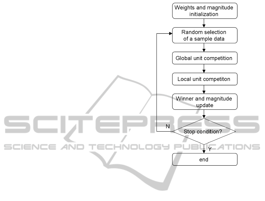
The next subsections describe the algorithm,

which ﬂowchart is shown in ﬁgure 1.

2.1 Initialization

M unit weights are initialized with data inputs ran-

domly selected from the dataset (with N samples).

Then the Magnitude Function MF(i,t) is calculated

from this initial codeword.

2.2 Random Selection of Data Samples

A sample data x(t) = (x

,. .. ,x

) ∈ ℜ

is randomly

selected at time t from the dataset. This process will

be repeated until every data has been presented to the

MSCL neural network. It is worth mentioning that it

is recommended to retrain the neural network several

cycles with the whole dataset to make results indepen-

dent from data-presentation ordering.

2.3 Global Unit Competition

In the ﬁrst step, K units (K = min(d+1,N)) with min-

imum distance from their weights to the input data

vector are selected. These units form the set:

S = {w

} ∨ kx(t) − w

(t)k < kx(t) − w

(t)k ∀i /∈ S

(1)

2.4 Local Unit Competition

Next, the winner unit j belonging to S which mini-

mizes the product of its Magnitude Function and the

distance of its weights to input data vector is selected:

j = argmin

(MF(k,t)kx(t) − w

(t)k) ∀k ∈ S (2)

FocusedImageColorQuantizationusingMagnitudeSensitiveCompetitiveLearningAlgorithm

517

2.5 Winner Updating

Only winner’s weights are iteratively adjusted for

each training sample as follows:

(t + 1) = w

(t) + α(t)(x(t) − w

(t)) (3)

where α(t) = α

ini

(α

final

/α)

t/T

is the learning factor

forced to decay with iteration time (t = {1,...,T}),

being α

ini

and α

final

constants.

Afterwards, the new magnitude function MF( j,t)

is calculated from this codeword. It is important to

avoid null values for the magnitude function other-

wise the competition will be distorted. Although an

on-line training is preferred, because it is more likely

to avoid local minima in contrast to batch methods,

when the cost of the magnitude calculation is high the

processing time can be reduced by updating the mag-

nitude only once per epoch.

2.6 Stopping Condition

Training is stopped when a termination condition is

reached. It may be the situation when all data sam-

ples have been presented to the MSCL neural network

along certain number of cycles (if a limited number of

samples is used), or the condition of low mean change

in unit weights, or any other function that could mea-

sure the training stabilization.

3 APPLICATIONS

In the following examples, data samples are 3D vec-

tors corresponding to the RGB components of the im-

age pixels. We have used the RGB space in order to

have comparable results to other works. The general

purpose is to get a reduced color palette to represent

the colors in the image paying attention to different

objectives. The next ﬁve examples show that, ade-

quately selecting the magnitude function, it is possi-

ble to get an optimal palette according to the desired

application.

3.1 Homogeneous Color Quantization

First example shows the case we call Homogeneous

Color Quantization. The mean quantization error

err

) for all samples within the Voronoi region of

unit i is used as magnitude function. The Q

err

for

sample x is the distance between x and its correspond-

ing best matching unit. This Magnitude forces the

palette colors to be uniformly distributed over the data

distribution in the RGB space independently of its

Figure 1: MSCL ﬂowchart.

data density. We use the known Tiger, Lena and Ba-

boon images for performance comparison in CQ tasks

(marked in tables as T*, L* and B*, where * is the

number of colors). Homogeneous MSCL (M-h) and

Centered MSCL (M-c, explained in subsection 3.2)

are compared against the most successful neural mod-

els used in different papers: SOM, FSCL, FCM, FS-

SOM, ADU and SGONG. The number of units is the

desired color-palette size. Training process applied

learning rates between (0.7-0.01) along three cycles,

except in ADU which algorithm parameters selection

follows (Uchiyama and Arbib, 1994). The threshold

for adding/removing a neuron used in SGONG was

(0.1/0.05).

Figure 2 shows the color reduction effects for tiger

image with ADU, Homogeneous MSCL and Cen-

tered MSCL (Only Tiger image is represented due to

space limitation). Table 1 shows the average Mean

Squared Error (MSE) for ten trials with different num-

ber of palette colors (8, 16 and 32). Peak Signal-

to-Noise Ratio (PSNR) measure can be easily calcu-

lated from MSE value. In general, ADU outperforms

all other models, closely followed by SOM and FS-

SOM. However, it is clear that ADU (top-right image

in ﬁgure 2) paints the tiger skin with greenish color

as an effect of the over-representation of green colors.

Both MSCL results (bottom images in ﬁgure 2) tend

IJCCI2012-InternationalJointConferenceonComputationalIntelligence

518

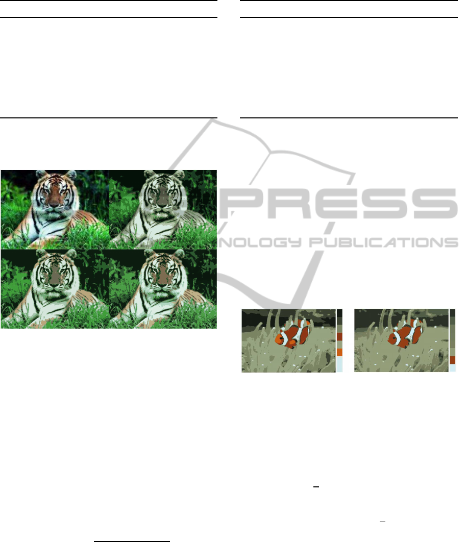
Table 1: MSE calculated in the whole image (ex. 1 and 2).

Image Som FSCL M-h FCM FSSom ADU M-c Sgong

T8 987 1016 1037 1005 985 990 1095 987

T16 566 596 577 606 564 562 667 570

T32 334 343 341 357 328.1 327.8 409 574

L8 401 416 424 451 400.2 406 406 400.9

L16 216 234 215 234 216 214 217 218

L32 121 126 122 141 120 119 125 222

B8 1120 1126 1138 1151 1117 1126 1227 1121

B16 633 641 633 693 632.4 632.8 751 635

B32 380 389 380 440 375.2 375.9 479 442

to maintain orange colors in the tiger skin, as they are

not focused on data density representation.

Figure 2: Original Tiger image (top-left) and its reconstruc-

tion using 8 colors applying: ADU (top-right), Homoge-

neous MSCL (bottom-left) and Centered MSCL (bottom-

right).

3.2 CQ Focused in the Image Center

Previous example provides a CQ task giving equal

importance to every pixel of the image, and not dis-

tinguishing between pixels of the foreground or the

background. However the more interesting image re-

gions usually are located in the foregroundcenter. Us-

ing MSCL with the adequate magnitude function is

possible to get a palette with colors mainly adapted to

pixels located in the foreground. In this example we

use the following magnitude function:

MF(i,t) =

∑

(1− d(x

(t)))

(t)

(4)

Where x

(t) are the data samples belonging to the

Voronoi region V

(t) of unit i at time t, and d(x

(t))

is the normalized distance, in the plane of the im-

age, calculated from the corresponding pixel position

to the center of the image. We compare the perfor-

mance of Centered MSCL (focused on image center),

Table 2: MSE calculated in the image center (ex. 1 and 2).

Image Som FSCL M-h FCM FSSom ADU M-c Sgong

T8 1223 1311 1207 1263 1214 1244 1151 1226

T16 626 710 596 735 631 608 485 655

T32 361 381 356 408 353 355 283 407

L8 445 472 436 552 440 447 423 447

L16 265 294 273 301 262 266 254 267

L32 161 167 160 187 159 159 149 163

B8 1346 1354 1210 1421 1343 1338 1062 1321

B16 708 740 683 833 705 689 602 714

B32 381 412 387 515 372 374 354 539

with the same methods used in previous example. The

number of colors and training parameters were also

the same.

M-c column of Table 1 shows the resulting aver-

age MSE using Centered MSCL for the whole im-

ages. Prototypes tend to focus on colors in the central

part of the image so, the MSE for the whole image is

worse than those obtained using other methods since

the background is under-represented. However, when

repeating the measures in the central area of the image

(150x170 pixels), this algorithm outperforms the oth-

ers because its color palette models mainly the central

region of the image. Table 2 shows the resulting MSE

values in central image area for all methods.

Figure 3: Fish example using MSCL (left) and FSCL (right)

with 8-color palette.

3.3 CQ Avoiding Mean Color

Some images present dominant background colors

with a few very different colors appearing in little de-

tails. The magnitude function deﬁned in this exam-

ple forces units to avoid the greyish mean color of

the whole image (

x), so other color regions are repre-

sented in more detail:

MF(i,t) = kw

(t) −

x(t)k (5)

Figure 3 represents the image with the reduced

color palette for MSCL (left) and FSCL (right), and

their corresponding color palettes. MSCL obtained

a more vivid color representation that includes three

greyish greens, two orange colors, two clear colors

and one stronger black, while FSCL tends to concen-

trate the units in the most common colors, showing

ﬁve greyish greens.

FocusedImageColorQuantizationusingMagnitudeSensitiveCompetitiveLearningAlgorithm

519

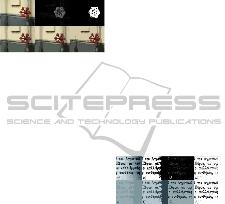
Figure 4: Saliency example. Top row, from left to right:

Original image, saliency map (clearer values for high

saliency), the mask binary image used for MSE measure-

ment and (bottom row, from left to right) the reconstructed

image with an 8-colors palette from: SOM, FS-SOM and

MSCL focused on the saliency.

3.4 CQ Focused in Salient Colors

The aim of salient feature detection is to ﬁnd distinc-

tive local events in images. Some works exploit the

possibilities of color distinctiveness in salient detec-

tion, (Vazquez et al., 2010). This example shows the

MSCL algorithm generating a color palette focused

on those salient regions. The chosen magnitude func-

tion is the mean computational global saliency as de-

ﬁned in (Vazquez et al., 2010). The magnitude is nor-

malized by the maximum, and varies from one to val-

ues close to zero in zones with low saliency (see im-

age in Figure 4 in the middle of the top row). We

used 8 colors with decreasing learning rates between

0.7 and 0.01 for every algorithm.

Figure 4 shows the results. The ﬁrst two algo-

rithms (SOM, FS-SOM) only obtain a red color and

present higher MSE values (SOM: 103.21 and FS-

SOM: 103.07) in those pixels belonging to the white

mask region of saliency (third top image of ﬁgure 4).

However, using the global saliency (second top image

of ﬁgure 4) as the magnitude for MSCL, the resulting

image shows three red variants and the MSE error is

lower (87.5). It is worth noticing that some other col-

ors are under-represented, which constitutes a minor

problem if the goal is to highlight the salient regions

of the image.

3.5 Image Binarization

The binarization of a text grey-scale image is a pro-

cess where each pixel in a image is converted into one

bit ’1’ or ’0’ depending upon whether the pixel cor-

responds to the text or the background. First row of

Figure 5a shows the image of a badly illuminated doc-

ument (image a), and the results of applying classical

binarization algorithms: Otsu method (b), ﬁltering of

original image with Laplacian operator (c) and its bi-

narization with Otsu (d). Otsu Method deﬁnitely fails

to get an adequate binarization because of the dark

grey values in the right margin of the paper. Filter-

ing with Laplacian operator provides a better result,

because it is an edge extraction mask. However, this

method does not ﬁll the letters. Competitive learn-

ing can be used for this application by training 2 units

to represent two levels of gray-scale, which should

correspond to the background and foreground classes.

Second row of ﬁgure 5 shows the results with: (e)

SOM, (f) MSCL in homogeneous grey quantization,

(g) MSCL with two features (further explained), and

(h) Otsu binarization of last example. The applica-

tion of MSCL with only two neurons, as shown in (f),

is equivalent to the Otsu Method because when us-

ing as mean of the data the unit weights representing

the class, the mean quantization error for each unit is

proportional to the standard deviation of the class.

The quantization result can be improved by using

as input a combination of the gray-level values and

the result of Laplace ﬁltering. Therefore data samples

will be two dimensional vectors combining the values

of both features. So, if we apply MSCL using homo-

geneous quantization we will get the two-level image

(g) and the corresponding binarized image (h). This

result is better than those achieved by other classical

methods.

Figure 5: Binarization example: in top row (a) original im-

age, (b) Otsu method, (c) ﬁltering with Laplacian operator,

and (d) its binarization with Otsu; in bottom row (e) SOM,

(f) MSCL in homogeneous grey quantization, (g) MSCL

with two features, and (h) Otsu binarization of (g).

4 CONCLUSIONS

This paper has shown the capabilities of the MSCL

algorithm for Color Quantization. MSCL is a neural

competitivelearning algorithm including a magnitude

function as a factor of the measure used for the unit

competition. The magnitude factor is a unit param-

eter calculated from any user-deﬁned function deal-

ing with the unit parameters or the data that it cap-

tures. The competitive process is executed in a two-

step comparison, ﬁrst step is as usual a competitive

IJCCI2012-InternationalJointConferenceonComputationalIntelligence

520

learning method using distances to selected K win-

ners, and in the second step those K units compare

their distances factorized by their magnitude values.

The model is parallel and can be executed on-line.

MSCL is compared with other VQ approaches in

four examples of image color quantization with dif-

ferent goals: focused on image foreground, avoiding

mean color, focused on saliency and text image bina-

rization. The results show that MSCL is more versa-

tile than other competitivelearning algorithms mainly

focused on density representations. MSCL forces the

units to distribute their color prototypes following any

desired property expressed by the appropriate magni-

tude of the data image. So, MSCL selects more colors

in the palette to accurately represent certain interest-

ing zones of the image, or generates palettes focused

on less represented, but interesting colors.

ACKNOWLEDGEMENTS

This work is partially supported by Spanish Grant

TIN2010-20177 (MICINN) and FEDER and by the

regional government DGA-FSE.

REFERENCES

Ahalt, S., Krishnamurthy, A., Chen, P., and Melton, D.

(1990). Competitive learning algorithms for vector

quantization. Neural networks, 3(3):277–290.

Atsalakis, A. and Papamarkos, N. (2006). Color reduc-

tion and estimation of the number of dominant col-

ors by using a self-growing and self-organized neu-

ral gas. Engineering Applications of Artiﬁcial Intelli-

gence, 19(7):769–786.

Bezdek, J. (1981). Pattern recognition with fuzzy objective

function algorithms. Plenum Press.

Bishop, C., Svens´en, M., and Williams, C. (1998). GTM:

The generative topographic mapping. Neural compu-

tation, 10(1):215–234.

Celebi, M. (2009). An effective color quantization method

based on the competitive learning paradigm. In Pro-

ceedings of the International Conference on Image

Processing, Computer Vision, and Pattern Recogni-

tion, IPCV, volume 2, pages 876–880.

Celebi, M. (2011). Improving the Performance of K-

Means for Color Quantization. Image (Rochester,

N.Y.), 29(4):260–271.

Celebi, M. and Schaefer, G. (2010). Neural Gas Clustering

for Color Reduction. In Proceedings of the Interna-

tional Conference on Image Processing, Computer Vi-

sion, and Pattern Recognition, IPCV, volume 1, pages

429–432.

Chang, C., Xu, P., and Xiao, R. (2005). New adaptive color

quantization method based on self-organizing maps.

Neural Networks, IEEE, 16(1):237–249.

Cheng, G., Yang, J., Wang, K., and Wang, X. (2006). Im-

age Color Reduction Based on Self-Organizing Maps

and Growing Self-Organizing Neural Networks. 2006

Sixth International Conference on Hybrid Intelligent

Systems (HIS’06), pages 24–24.

Dekker, A. (1994). Kohonen Neural Networks for Optimal

Colour Quantization. Network: Computation in Neu-

ral Systems, 3(5):351–367.

Durbin, R. and Willshaw, D. (1987). An analogue approach

to the travelling salesman problem using an elastic net

method. Nature, 326(6114):689–691.

Itti, L. and Koch, C. (2001). Computational modeling

of visual attention. Nature reviews neuroscience,

2(3):194–203.

Koch, C. and Ullman, S. (1985). Shifts in selective visual

attention: towards the underlying neural circuitry. Hu-

man Neurobiology, 4(4):219–227.

Kohonen, T. (2001). Self-Organizing Maps. Springer.

Lazaro, J., Arias, J., Martin, J., Zuloaga, A., and Cuadrado,

C. (2006). SOM Segmentation of gray scale images

for optical recognition. Pattern Recognition Letters,

27(16):1991–1997.

Lloyd, S. (1982). Least squares quantization in PCM. IEEE

Transactions on Information Theory, 28(2):129–137.

Martinetz, T., Berkovich, S., and Schulten, K. (1993).

‘Neural-gas’ network for vector quantization and its

application to time-series prediction. IEEE Transac-

tions on Neural Networks, 4(4):558–569.

Nikolaou, N. and Papamarkos, N. (2009). Color reduction

for complex document images. International Journal

of Imaging Systems and Technology, 19(1):14–26.

Papamarkos, N. (2003). A neuro-fuzzy technique for doc-

ument binarisation. Neural Computing and Applica-

tions, 12(3-4):190–199.

Pelayo, E., Buldain, D., and Orrite, C. (2012). Magnitude

Sensitive Competitive Learning. In 20th European

Symposium on Artiﬁcial Neural Networks, Comp. Int.

and Machine Learning, volume 1, pages 305–310.

Treisman, A. and Gelade, G. (1980). A feature integration

theory of attention. Cognitive Psychology, 12:97–136.

Uchiyama, T. and Arbib, M. (1994). Color image seg-

mentation using competitive learning. IEEE Trans-

actions on Pattern Analysis and Machine Intelligence,

16(12):1197–1206.

Vazquez, E., Gevers, T., Lucassen, M., van de Weijer,

J., and Baldrich, R. (2010). Saliency of color im-

age derivatives: a comparison between computational

models and human perception. Journal of the Opti-

cal Society of America. A, Optics, image science, and

vision, 27(3):613–21.

Xu, L., Krzyzak, A., and Oja, E. (1993). Rival Penalized

Competitive Learning for Clustering Analysis, RBF

net and Curve Detection. IEEE Tr. on Neural Net-

works, 4:636–649.

FocusedImageColorQuantizationusingMagnitudeSensitiveCompetitiveLearningAlgorithm

521