Bayesian Regularized Committee of Extreme Learning Machine
Jos´e M. Mart´ınez-Mart´ınez, Pablo Escandell-Montero, Emilio Soria-Olivas, Joan Vila-Franc´es
and Rafael Magdalena-Benedito
IDAL, Intelligent Data Analysis Laboratory, Electronic Engineering Department, University of Valencia,
Av de la Universidad, s/n, 46100, Burjassot, Valencia, Spain
Keywords:
Extreme Learning Machine, Committee, Bayesian Linear Regression.
Abstract:
Extreme Learning Machine (ELM) is an efficient learning algorithm for Single-Hidden Layer Feedforward
Networks (SLFNs). Its main advantage is its computational speed due to a random initialization of the param-
eters of the hidden layer, and the subsequent use of Moore-Penrose’s generalized inverse in order to compute
the weights of the output layer. The main inconvenient of this technique is that as some parameters are ran-
domly assigned and remain unchanged during the training process, they can be non-optimum and the network
performance may be degraded. This paper aims to reduce this problem using ELM committees. The way to
combine them is to use a Bayesian linear regression due to its advantages over other approaches. Simulations
on different data sets have demonstrated that this algorithm generally outperforms the original ELM algorithm.
1 INTRODUCTION
A simple and efficient learning algorithm for
Single-Hidden Layer Feedforward Neural Networks
(SLFNs), called Extreme Learning Machine (ELM),
has been recently proposed in (Huang et al., 2006).
ELM has been successfully applied to a number of
real world applications (Sun et al., 2008; Malathi
et al., 2010), showing a good generalization perfor-
mance with an extremely fast learning speed. How-
ever, an issue with ELM is that as some parameters
are randomly assigned and remain unchanged during
the training process, they can be non-optimumand the
network performance may be degraded. It has been
demonstrated that combining suboptimal models is an
effective and simple strategy to improve the perfor-
mance of each one of the combination members (Seni
and Elder, 2010).
There are different ways to combine the output
of several models (Seni and Elder, 2010). The sim-
plest way of combining models is to take a linear
combination of their outputs. Nonetheless, some re-
searchers have shown that using some instead of all
the available models can provide better performance.
In (Escandell-Montero et al., 2012), regularization
methods are used such as Ridge regression (Hoerl and
Kennard, 1970), Lasso (Tibshirani, 1996) and Elastic
Net (Zou and Hastie, 2005) in order to select the mod-
els, and the proportion of these, that should be part of
the committee.
This paper aims to investigate the use of bayesian
linear regression regularization in order to build the
committee. The use of this kind of regression involves
three main advantages (Bishop, 2007):
1. Regularization. This kind of regression involves a
regularization term whose associated parameter is
calculated automatically.
2. Calculation of the confidence intervals of the out-
put without the need of applying methods that are
computationally intensive, e.g. bootstrap.
3. Introduction of knowledge. Bayesian methods al-
low the introduction of a priori knowledge of the
problem
The remaining of this paper is organized as fol-
lows. Section 2 briefly presents the ELM algorithm.
The details of the proposed method are described in
Section 3. Results and discussion are presented in
Section 4. Finally, Section 5 summarizes the conclu-
sions of the present study.
2 EXTREME LEARNING
MACHINE
ELM was proposed by Huang et al. (Huang et al.,
2006). This algorithm makes use of the SLFN ar-
chitecture. In (Huang et al., 2006), it is shown that
109
M. Martínez-Martínez J., Escandell-Montero P., Soria-Olivas E., Vila-Francés J. and Magdalena-Benedito R. (2013).
Bayesian Regularized Committee of Extreme Learning Machine.
In Proceedings of the 2nd International Conference on Pattern Recognition Applications and Methods, pages 109-114
DOI: 10.5220/0004173901090114
Copyright
c
 SciTePress

the weights of the hidden layer can be initialized ran-
domly, thus being only necessary the optimization of
the weights of the output layer. That optimization can
be carried out by means of the Moore-Penrose gen-
eralized inverse. Therefore, ELM allows reducing the
computational time needed for the optimization of the
parameters due to fact that is not based on gradient-
descent methods or global search methods.
Let be a set of N patterns, D = (x
i
, o
i
);i = 1. . . N,
where {x
i
} ∈ R
d
1
and {o
i
} ∈ R
d
2
, so that the goal is
to find a relationship between x
i
and o
i
. If there are M
nodes in the hidden layer, the SLFN’s output for the
j-th pattern is given by y
j
:
y
j
=
M
∑
k=1
h
k
· f (w
k
, x
j
) (1)
where 1 ≤ j ≤ N, w
k
stands for the parameters of the
k-th element of the hidden layer (weights and biases),
h
k
is the weight that connects the k-th hidden element
with the output layer and f is the function that gives
the output of the hidden layer; in the case of MLP, f is
an activation function applied to the scalar product of
the input vector and the hidden weights. The SLFN’s
output can be expressed in matrix notation as
y = G· h, where h is the vector of weights of the out-
put layer, y is the output vector and G is given by:
G =



f (w
1
, x
1
) . . . f (w
M
, x
1
)
.
.
.
.
.
.
.
.
.
f (w
1
, x
N
) ··· f (w
M
, x
N
)



(2)
As mentioned previously, ELM proposes a random
initialization of the parameters of the hidden layer,
w
k
. Afterwards the weights of the output layer are
obtained by the Moore-Penrose’s generalized inverse
(Rao and Mitra., 1972) according to the expression
h = G
†
· o, where G
†
is the pseudo-inverse matrix.
3 BAYESIAN REGULARIZED
ELM COMMITTEE
3.1 Ensemble Methods
A committee, also known as ensemble, is a method
that consists in taking a combination of several mod-
els to form a single new model (Seni and Elder, 2010).
In the case of a linear combination, the commit-
tee learning algorithm tries to train a set of models
{s
1
, . . . , s
P
} and choose coefficients {m
1
, . . . , m
P
} to
combine them as y(x) =
∑
P
i=1
m
i
s
i
(x). The output of
the committee on instance x
i
is computed as
y(x
i
) =
P
∑
k=1
m
k
s
k
(x
i
) = s
T
i
m, (3)
where s
i
= [s
1
(x
i
), . . . , s
P
(x
i
)]
T
are the predictions of
each committee member.
The main idea of the proposed method lies in com-
puting the coefficients that combine the committee
members using a bayesian linear regression.
3.2 Bayesian Linear Regression
Any Bayesian modeling is carried out in two steps
(Congdon, 2006):
• Inference of the posterior distribution of the
model parameters. It is proportional to the prod-
uct of the prior distribution and the likelihood
function: P(w|D) ∝ P(w) · P(D|w) where w is
the set of parameters and D is the data set.
• Calculation of the output distribution of the
model, y
new
(only one output is considered for the
sake of simplicity), for a new input x
new
. It is de-
fined as the integral of the posterior distribution of
the parameters w:
p(y
new
|x
new
, D) =
Z
p(y
new
|x
new
, w)· p(w|D)·dw
(4)
Equation (4) constitutes a natural way of esti-
mating the confidence interval of the model output
(Bishop, 2007).
The linear model follows this relationship:
y = h
T
· x+ ε (5)
where ε follows a normal distribution with zero mean
and variance σ
2
, N(0;σ
2
). Equation (5) leads to the
definition of the conditional distribution:
p(y|x, h, σ
2
) = N (h
T
· x;σ
2
) (6)
In most applications, the parameter distribution is
considered to be (Bishop, 2007):
p(h|α) = N (0;α
−1
· I) (7)
where I is the identity matrix and α an hyperparame-
ter. Assuming that the prior distribution and the likeli-
hood function follow Gaussian distributions, the pos-
terior distribution is also Gaussian, with a mean value
m and a variance S defined as (Bishop, 2007; Chen
and Martin, 2009):
m = σ
−2
· S· X
T
· y (8)
S =

αI+ σ
−2
· X
T
· X

−1
(9)
where y = [y
1
, y
2
, . . . , y
N
] and X = [x
1
, x
2
, . . . x
N
] are
the matrix with the model output vectors and the input
vector for those values, respectively.
ICPRAM2013-InternationalConferenceonPatternRecognitionApplicationsandMethods
110

It is worth noting that the regularization term α
in (9) is a natural consequence of the Gaussian ap-
proach (Bishop, 2007). This fact differs from other
approaches, which requires a term on the cost func-
tion being minimized (Deng et al., 2009). Param-
eters from (9) and (8) are optimized iteratively by
means of the ML-II (Berger., 1985) or Evidence Pro-
cedure (Barber, 2012). This process applies itera-
tively expressions (8), (9), (10), (11) and (12); where
N is the number of parameters and P is the number of
patterns (Bishop, 2007) :
γ = N − α · trace[S] (10)
α =
γ
m
T
m
(11)
σ
2
=
∑
P
i=0

y
i
− m
T
· x
i

2
P− γ
(12)
The iterative process is stopped when the differ-
ence of the norm of m between successive iterations
falls below a given value. The posterior distribu-
tion of the parameters can be applied to (4) in or-
der to obtain the output y
new
given a new input x
new
.
The output follows a distribution p(y
new
|y, α, σ
2
) =
N

h
T
· x
new
;σ
2
(x
new
)

; where the variance is defined
as (Bishop, 2007; Chen and Martin, 2009):
σ
2
(x
new
) = σ
2
+ x
T
new
· S· x
T
new
(13)
Summing up, using a Gaussian approach in the
linear step of the model gives the following advan-
tages (Bishop, 2007; Chen and Martin, 2009; Cong-
don, 2006):
• Regularization. The Bayesian approach involves
the use of some parameters (hyperparameters)
that allow regularization. This regularization term
is obtained from the distribution of the model pa-
rameters and helps reducing the overfitting of the
model (Bishop, 2007), as we will show in Section
4.
• Confidence Intervals. The use of CIs increases the
reliability of a model’s output. When using neu-
ral models, CIs are usually obtained after training
the model by means of methods that tend to be
computationally costly, e.g. bootstrap (Alpaydin,
2010). The proposed method allows the calcu-
lation of CIs and the weight optimization at the
same time. This intervals can be calculated easily
with the S matrix (9), the input matrix and with
the noise variance that is computed during the it-
erative calculation of the weights (Barber, 2012).
• A Priori Knowledge. A priori knowledge can be
introduced in the models by means of error dis-
tributions and parameter distributions that must
be defined when applying Bayes’ theorem. This
knowledge can improve the performance of the
model.
4 EXPERIMENTAL RESULTS
Several benchmark problems were chosen for the ex-
periments. The data sets were collected from the Uni-
versity of California at Irvine (UCI) Machine Learn-
ing Repository
1
and they were chosen due to the over-
all heterogeneity in terms of number of samples and
number of variables. The different attributes for the
data sets are summarized in Table 1.
Table 1: Data sets used for the experiments.
Data sets Samples Attributes
Housing 506 13
Delta elvevators 9517 6
Abalone 4177 8
Auto 392 7
Autoprice 159 15
Parkinson 5875 21
Add10 9792 10
The performance of the proposed approach was
evaluated for the previous data sets. We used the
following methodology in order to achieve a relative
comparison among the several methods:
1. The parameters of the hidden layer of the SLFN
were obtained randomly in 50 experiments. The
inputs and outputs of the model were standardized
(zero mean and unity variance).
2. The number of hidden neurons of each ELM was
varied from 20 to 100 neurons with an increment
of 20 neurons.
3. For the number of committee members, the same
strategy was carried out; committee members
from 20 to 100 ELMs were considered with incre-
ments of 20 for every different ELM architecture.
4. Two kinds of committees have been tested in this
work. On one hand, a linear combination has been
proposed, where the coefficients are calculated by
least squares. On the other hand, the bayesian lin-
ear combination previously stated.
5. In the seven tackled problems, the training data
set was formed by 50% of the patterns, and the re-
maining 50% were used for validation purposes.
1
http://archive.ics.uci.edu/ml/
BayesianRegularizedCommitteeofExtremeLearningMachine
111

20 30 40 50 60 70 80 90 100
0.26
0.28
0.3
0.32
0.34
0.36
0.38
Number of hidden nodes
MAE
Min.
LS
Bayesian
(a) MAE for a committee composed of 20 members.
20 30 40 50 60 70 80 90 100
0.26
0.28
0.3
0.32
0.34
0.36
0.38
Number of hidden nodes
MAE
Min.
LS
Bayesian
(b) MAE for a committee composed of 40 members.
20 30 40 50 60 70 80 90 100
0.26
0.28
0.3
0.32
0.34
0.36
0.38
0.4
Number of hidden nodes
MAE
Min.
LS
Bayesian
(c) MAE for a committee composed of 60 members.
20 30 40 50 60 70 80 90 100
0.25
0.3
0.35
0.4
0.45
Number of hidden nodes
MAE
Min.
LS
Bayesian
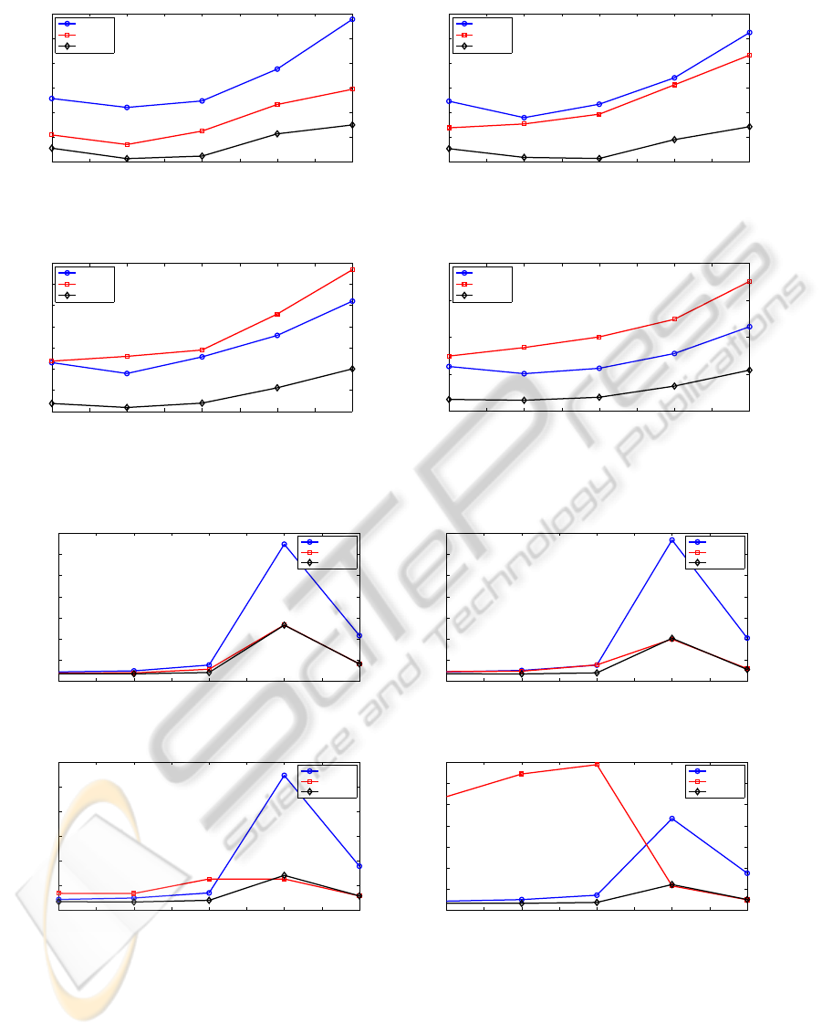
(d) MAE for a committee composed of 80 members.
Figure 1: Performance in terms of MAE in the validation set of the proposed algorithm compared with the linear comittee of
ELMs and with the member of the committee which presented the minimum error for Abalone data set.
20 30 40 50 60 70 80 90 100
0
1
2
3
4
5
6
7
Number of hidden nodes
MAE
Min.
LS
Bayesian
(a) MAE for a committee composed of 20 members.
20 30 40 50 60 70 80 90 100
0
1
2
3
4
5
6
7
Number of hidden nodes
MAE
Min.
LS
Bayesian
(b) MAE for a committee composed of 40 members.
20 30 40 50 60 70 80 90 100
0
1
2
3
4
5
6
Number of hidden nodes
MAE
Min.
LS
Bayesian
(c) MAE for a committee composed of 60 members.
20 30 40 50 60 70 80 90 100
0
1
2
3
4
5
6
7
Number of hidden nodes
MAE
Min.
LS
Bayesian
(d) MAE for a committee composed of 80 members.
Figure 2: Performance in terms of MAE in the validation set of the proposed algorithm compared with the linear comittee of
ELMs and with the member of the committee which presented the minimum error for Autoprice data set.
Each pattern was assigned randomly to one of the
two sets (either training or validation) for each ex-
periment.
Table 2 shows the performance in terms of MAE
(Mean Absolute Error) in the validation set of the pro-
posed method, the bayesian regularized ELM com-
mittee (Bayes.), in comparison with the results of the
linear committee (LS), where the coefficients are cal-
culated by least squares as previously mentioned. The
MAE was computed according with (14):
ICPRAM2013-InternationalConferenceonPatternRecognitionApplicationsandMethods
112

MAE =
1
N
N
∑
i=1
|y
i
− ˆy
i
| (14)
where y
i
is the observed output and ˆy
i
is the output
predicted by the model.
Another model is included in Table 2 (Min.),
which refers to the minimum MAE of the ELM net-
work inside the whole committee of ELMs, that is, the
member of the committee which presented the mini-
mum MAE. In this way, we obtain a reference value
that indicates if the committee provides best results as
a whole than the best ELM network that takes part of
the committee.
Table 2 shows the median value of the 50 experi-
ments that were considered for each configuration of
ELM-committee. Moreover, only three of the five val-
ues of the different number of neurons in the hidden
layer tested are presented for the sake of simplicity.
This values are 20, 60, 100 initial number of neurons,
which corresponds with first, second and third rows of
each method respectively (Table 2). The columns cor-
responds to the several number of committee mem-
bers tested, which were varied from 20 to 100 with
increments of 20, as mentioned previously.
To summarize the information contained in Table
2, a comparison of three methods has been carried
out. To do such comparison, the value of the MAE
in each method, for each number of committee tested
(columns) and each number of hidden neurons tested,
is compared. The result of this comparison shows
that, in general terms, the proposed method outper-
form the other two methods. Specifically, the 71.43%
of the times the proposed method won, the 9.52% of
the times the linear committee won and the 19.05% of
the times they tied. The third method, the member of
the committee which presented the minimum MAE,
never was the best method.
In order to illustrate the performance of the pro-
posed algorithm, graphically, compared with the lin-
ear comittee of ELMs and with the member of the
committee which presented the minimum error, we
present Figures 1 and 2. These figures show the re-
sults for Abalone (Figure 1) and Autoprice (Figure 2)
data sets. Each figure presents four cases that cor-
respond to several committees. The first case corre-
sponds to a committee composed of 20 members, the
second case to one of 40 members, the third case to
one of 60 members and, finally, the latter case corre-
sponds to a committee composed of 80 members.
Notice that for Abalone data set, Figures 1a and
1b the bayesian regularized ELM committee presents
always the minimum MAE; the second best method
is the linear committee of ELM. However, Figures 1c
and 1d show that the proposed method presents al-
ways the minimum MAE again, but in these cases (60
Table 2: Performance in terms of MAE in the validation set
of the proposed method (Bayes.), in comparison with the
results of the linear committee (LS) and the member of the
committee which presented the minimum MAE.
Data set Method C1 C2 C3 C4 C5
0,311 0,309 0,306 0,310 0,309
Min. 0,309 0,307 0,311 0,308 0,312
0,376 0,365 0,364 0,364 0,364
Abalone 0,282 0,288 0,307 0,324 0,371
LS 0,285 0,299 0,318 0,350 0,388
0,319 0,347 0,394 0,425 0,486
0,271 0,271 0,267 0,266 0,262
Bayes. 0,265 0,263 0,268 0,269 0,273
0,290 0,289 0,300 0,305 0,309
0,497 0,491 0,494 0,493 0,495
Min. 0,425 0,425 0,427 0,427 0,425
0,407 0,407 0,407 0,407 0,407
Add10 0,408 0,398 0,394 0,390 0,384
LS 0,375 0,361 0,348 0,339 0,331
0,353 0,336 0,323 0,313 0,301
0,408 0,398 0,394 0,389 0,383
Bayes. 0,375 0,361 0,348 0,338 0,331
0,353 0,336 0,323 0,313 0,301
0,311 0,309 0,306 0,310 0,309
Min. 0,309 0,307 0,311 0,308 0,312
0,376 0,365 0,364 0,364 0,364
Auto 0,282 0,288 0,307 0,324 0,371
LS 0,285 0,299 0,318 0,350 0,388
0,319 0,347 0,394 0,425 0,486
0,271 0,271 0,267 0,266 0,262
Bayes. 0,265 0,263 0,268 0,269 0,273
0,290 0,289 0,300 0,305 0,309
0,444 0,448 0,444 0,438 0,424
Min. 0,769 0,768 0,710 0,720 0,732
2,159 2,043 1,791 1,758 1,773
Autoprice 0,391 0,459 0,692 5,373 1,850
LS 0,571 0,776 1,273 6,883 1,791
0,822 0,599 0,587 0,504 0,505
0,359 0,356 0,356 0,335 0,341
Bayes. 0,416 0,399 0,410 0,379 0,397
0,822 0,560 0,587 0,515 0,505
0,480 0,477 0,479 0,477 0,477
Min. 0,463 0,462 0,463 0,462 0,461
0,460 0,459 0,460 0,459 0,459
Delta elev. 0,459 0,457 0,457 0,456 0,456
LS 0,455 0,454 0,455 0,455 0,455
0,453 0,454 0,455 0,455 0,456
0,459 0,456 0,456 0,454 0,453
Bayes. 0,454 0,453 0,453 0,452 0,451
0,453 0,453 0,453 0,452 0,452
0,439 0,440 0,440 0,441 0,438
Min. 0,415 0,408 0,410 0,403 0,406
0,422 0,412 0,420 0,419 0,416
Housing 0,374 0,376 0,383 0,390 0,388
LS 0,330 0,331 0,348 0,346 0,361
0,309 0,317 0,327 0,341 0,359
0,364 0,351 0,348 0,339 0,327
Bayes. 0,319 0,308 0,310 0,302 0,300
0,301 0,286 0,289 0,285 0,287
0,753 0,755 0,754 0,752 0,750
Min. 0,702 0,704 0,705 0,702 0,700
0,669 0,669 0,671 0,669 0,669
Parkinson 0,704 0,678 0,658 0,647 0,631
LS 0,633 0,616 0,605 0,592 0,589
0,594 0,581 0,574 0,565 0,560
0,705 0,679 0,659 0,648 0,633
Bayes. 0,633 0,617 0,606 0,592 0,589
0,593 0,582 0,575 0,565 0,558
and 80 committee members) the second best method
is Min. (the member of the committee which pre-
sented the minimum MAE).
For Autoprice data set, Figures 2a and 2b show
BayesianRegularizedCommitteeofExtremeLearningMachine
113

that the proposed method and the linear committee of
ELMs are very similar; although the proposed method
presents less MAE in some cases. However, Fig-
ures 2c and 2d show that, in general terms, the pro-
posed method presents the minimum MAE again, but
in these cases, when the number of hidden neurons is
60, the linear committee of ELMs presents less MAE,
although the difference is almost negligible, specially
in Figure 2c.
Summarizing, in general terms the proposed
method outperforms the linear comittee of ELMs and
the member of the committee which presented the
minimum MAE. Moreover, it presented more robust-
ness than the mentioned methods. This can be seen
in Figure 2d, where the only method that is almost
constant is the proposed one.
5 CONCLUSIONS
This paper aims to investigate the use of bayesian
linear regression regularization with the intention of
building a committee of ELM in order to avoid the
problem of local minima found in this emergent neu-
ral network. The use of this kind of regression in-
volves three main advantages:
1. Regularization. This kind of regression involves a
regularization term whose associated parameter is
calculated automatically.
2. Calculation of the confidence intervals of the out-
put without the need of applying methods that are
computationally intensive, e.g. bootstrap.
3. Introduction of knowledge. Bayesian methods al-
low the introduction of a priori knowledge of the
problem.
A performance comparison of this method with
the linear comittee of ELMs and with the member
of the committee which presented the minimum er-
ror has been carried out on widely used benchmark
problems of some real-world regression problems.
Summarizing, the proposed method not only
keeps the advantage of extremely fast training speed
but also solves the main inconvenient of this tech-
nique; the local minima problem. In general terms
the proposed method outperforms the linear comit-
tee of ELMs and the member of the committee which
presented the minimum MAE. Moreover, it presented
more robustness than the mentioned methods. An-
other advantage is that due to the fact that this method
uses a regularization method entails that the general-
ization ability improves.
REFERENCES
Alpaydin, E. (2010). Introduction to Machine Learning.
MIT Press, 2nd edition.
Barber, D. (2012). Bayesian Reasoning and Machine
Learning. Cambridge University Press.
Berger., J. O. (1985). Statistical Decision Theory and
Bayesian Analysis. Springer.
Bishop, C. M. (2007). Pattern Recognition and Machine
Learning. Springer, 1st ed. 2006. corr. 2nd printing
edition.
Chen, T. and Martin, E. (2009). Bayesian linear regres-
sion and variable selection for spectroscopic calibra-
tion. Anal. Chim. Acta, 631(1):13–21.
Congdon, P. (2006). Bayesian Statistical Modelling. Wiley.
Deng, W., Zeng, Q., and Chen, L. (2009). Proc. ieee symp.
comput. intell. data mining.
Escandell-Montero, P., Mart´ınez-Mart´ınez, J. M., Soria-
Olivas, E., Guimer´a-Tom´as, J., Mart´ınez-Sober, M.,
and Serrano-L´opez, A. J. (2012). Regularized com-
mittee of extreme learning machine for regression
problems. In European Symposium on Artificial Neu-
ral Networks, Computational Intelligence and Ma-
chine Learning, 2012. ESANN ’12.
Hoerl, A. E. and Kennard, R. W. (1970). Ridge regression:
Applications to nonorthogonal problems. Technomet-
rics, 12(1):69–82.
Huang, G., Zhu, Q.-Y., and Siew, C. (2006). Extreme learn-
ing machine: Theory and applications. Neurocomput-
ing, 70:489–501.
Malathi, V., Marimuthu, N., and Baskar, S. (2010). Intel-
ligent approaches using support vector machine and
extreme learning machine for transmission line pro-
tection. Neurocomputing, 73(10-12):2160 – 2167.
Rao, C. R. and Mitra., S. K. (1972). Generalized Inverse of
Matrices and Its Applications. Wiley.
Seni, G. and Elder, J. (2010). Ensemble Methods in
Data Mining: Improving Accuracy Through Combin-
ing Predictions. Morgan and Claypool Publishers.
Sun, Z.-L., Choi, T.-M., Au, K.-F., and Yu, Y. (2008). Sales
forecasting using extreme learning machine with ap-
plications in fashion retailing. Decision Support Sys-
tems, 46(1):411 – 419.
Tibshirani, R. (1996). Regression shrinkage and selection
via the lasso. Journal of the Royal Statistical Society
(Series B), 58:267–288.
Zou, H. and Hastie, T. (2005). Regularization and variable
selection via the elastic net. Journal of the Royal Sta-
tistical Society B, 67:301–320.
ICPRAM2013-InternationalConferenceonPatternRecognitionApplicationsandMethods
114