A New Method for Assessing the Exploratory Field of View (EFOV)

Enkelejda Tafaj

, Sebastian Hempel

, Martin Heister

, Kathrin Aehling

, Janko Dietzsch

Frank Schaeffel

, Wolfgang Rosenstiel

and Ulrich Schiefer

Wilhelm-Schickard Institute, Computer Engineering Department, University of T

ubingen, T

ubingen, Germany

Centre for Ophthalmology, Institute for Ophthalmic Research, University of T

ubingen, T

ubingen, Germany

Keywords:

Exploratory Field of View, Visual Exploration, Visual Field, Ophthalmology, Eye Movements.

Abstract:

Intact visual functioning is a crucial prerequisite for driving safely. Visual function tests usually include the

assessment of the visual acuity and binocular visual ﬁeld. Based on these results, persons suffering from

some types of visual ﬁeld defects that affect the central 20 degree region are prohibited from driving, although

they may have developed patterns of eye and head movements that allow them to compensate for their visual

impairment. We propose a new method to assess the exploratory ﬁeld of view (EFOV), i.e. the ﬁeld of view

of a subject when eye movements are allowed. With EFOV testing we aim at capturing the visual exploration

capability of a subject and thus understand the real impact of visual ﬁeld defects on activities of daily living

and potential compensatory strategies.

1 INTRODUCTION

Visual information accounts for up to 90% of driv-

ing related-inputs (Taylor, 1982). The assessment of

the visual acuity and visual ﬁeld are therefore impor-

tant elements of ability tests in trafﬁc ophthalmology.

According to current recommendations, subjects suf-

fering from binocular visual ﬁeld defects affecting the

central 20 degree region are prohibited from driving.

Visual ﬁeld testing, i.e. perimetry, consists of measur-

ing the sensitivity of visual perception as a function of

location in the visual ﬁeld (Schiefer et al., 2008). The

stimuli are projected onto a homogenous curved back-

ground. In kinetic perimetry, a stimulus with constant

luminance is moved from blind areas almost perpen-

dicularly towards the assumed visual ﬁeld defect bor-

der. The position at which the presented stimulus is

detected, represets the border and/or the outer limit of

the visual ﬁeld. Static perimetry is mainly performed

automatically by computer-driven stimulus presenta-

tion. The size and location of a stimulus is kept con-

stant while its luminance varies, usually in a stepwise

up- and-down manner. Subjects indicate stimulus per-

ception by pressing a response button. A missing re-

sponse to a stimulus projection is interpreted as a fail-

ure to seeing it (Schiefer et al., 2008).

Although perimetry is a highly standardized psy-

chophysical method, it is yet rather artiﬁcial. In ev-

eryday but safety critical activities such as driving a

car, subjects are usually neither confronted with

small, rather dim light stimuli on an homogeneous

background nor do they have to refrain from eye and

head movements. Instead, conspicuous objects within

the visual ﬁeld induce a shift of the visual attention,

eliciting eye and head movements towards the object

of interest. These types of movements can also help

to - at least partially - compensate for existing visual

defects. Several studies, e.g. (Martin et al., 2007),

(Hardiess et al., 2010), (Pambakian et al., 2000), (Ri-

ley et al., 2007), have been conducted to explore the

viewing behavior of persons with advanced visual

ﬁeld defects such as homonymous, where half of the

visual ﬁeld in both eyes is affected. These studies

conﬁrmed that persons who have developed a good

exploration capability are able, by performing efﬁ-

cient eye and head movements towards their visual

ﬁeld defect, to obtain information from the impaired

part of the visual ﬁeld. Present ability testing does

address ocular motility, however only with regard to

disclose double vision during smooth pursuit instead

of unveiling insufﬁcient saccadic eye movements to-

wards objects of interest.

In this paper we introduce a new method to assess

the exploratory ﬁeld of view (EFOV), i.e. the ﬁeld of

view of a person when eye movements are allowed.

During EFOV testing, the subject is encouraged to

move his eyes towards the presented stimulus in or-

der to ﬁxate it. EFOV testing can capture the visual

Tafaj E., Hempel S., Heister M., Aehling K., Dietzsch J., Schaeffel F., Rosenstiel W. and Schiefer U..

A New Method for Assessing the Exploratory Field of View (EFOV).

DOI: 10.5220/0004190600050011

In Proceedings of the International Conference on Health Informatics (HEALTHINF-2013), pages 5-11

ISBN: 978-989-8565-37-2

 2013 SCITEPRESS (Science and Technology Publications, Lda.)

exploration capability of a subject and thus reveal the

real impact of a visual ﬁeld defect. Implementation

details and exemplary results of the assessment of the

exploratory ﬁeld of view will be presented in the fol-

lowing sections.

2 THE EXPLORATORY FIELD OF

VIEW (EFOV) TEST

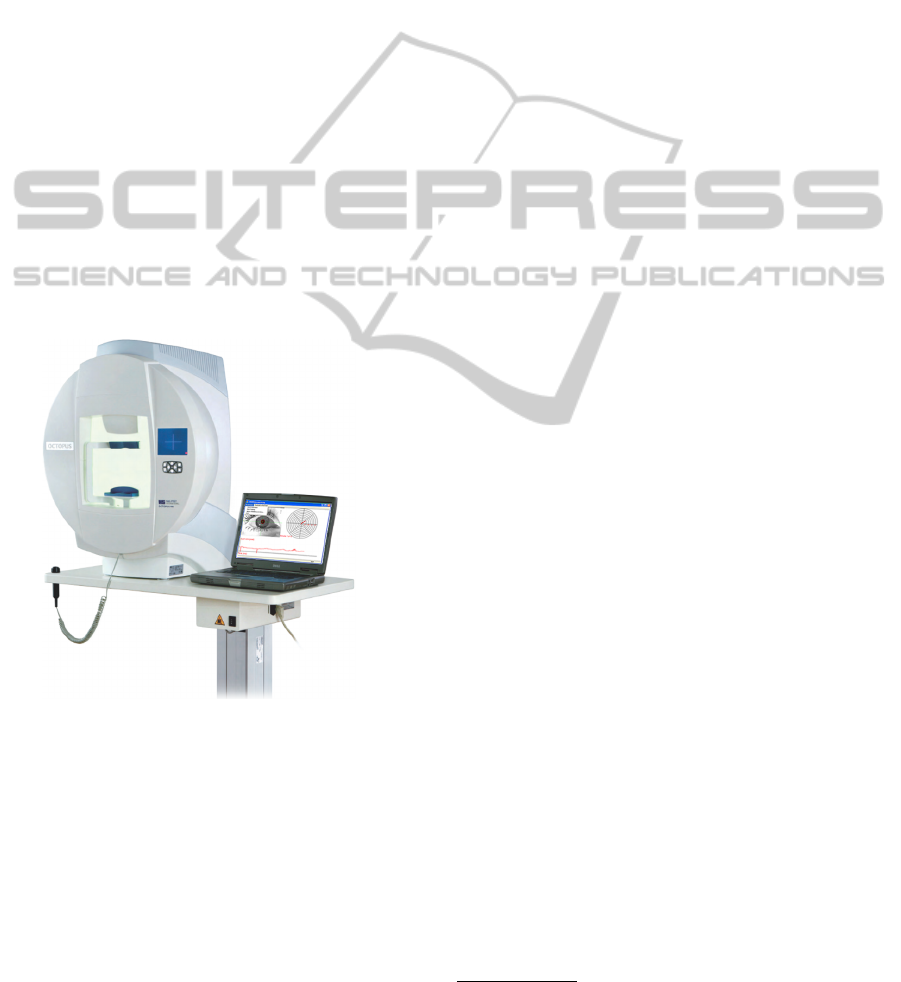
The Exploratory Field Of View (EFOV) Test is im-

plemented for usage with cupola perimeters such as

the Octopus 900 perimeter (HAAG-STREIT Inc., Ko-

eniz, Switzerland) depicted in Figure 1. The perimet-

ric system itself consists of an examination unit, Oc-

topus 900 cupola, and a control unit, Figure 1. The

control unit is a notebook computer or a PC that com-

municates with the examination element via an Ether-

net link. For ﬁxation stability, the Octopus perimeters

are equipped with a camera directed to the subject’s

eye. The eye is illuminated with infrared LEDs and

then captured by a CMOS camera at an image resolu-

tion of 320 × 240px and a sampling rate of 20Hz.

Figure 1: The EFOV test on an Octopus 900 perimeter.

The EFOV test is implemented as an add-on to the

Octopus control software. In contrast to usual peri-

metric examinations, where the subjects’ head and

eyes are ﬁxated, during the assessment of EFOV the

subject is allowed to move his eyes towards the pre-

sented stimulus and ﬁxate it. A stimulus is considered

as perceived if it is ﬁxated by the subject. Therefore,

no explicit subject’s response (e.g. by pressing a but-

ton) is needed. The examination procedure consists

of the following steps:

• Similar to conventional perimetric examinations,

ﬁrst the examination set-up is conﬁgured. This in-

cludes the choice of the grid of stimuli that will be

presented sequentially, as well as an initial param-

eter setting, e.g. the deﬁnition of a time windows

deﬁning the stimulus presentation time or for cap-

turing the user’s response.

• After the general conﬁguration of the examina-

tion, a calibration routine is started. During cali-

bration, a mapping between the eye position in the

camera image and the gaze position in the scene,

i.e. on the perimeter surface, is calculated. The

algorithms involved in this examination step will

be discussed in the next section.

• Once the calibration procedure is successful, the

examination can start. A grid of stimuli is loaded

and the stimuli are presented sequentially in ran-

dom order. For each stimulus the subject is en-

couraged to perform eye movements towards the

stimulus location in order to ﬁxate the target. The

software captures the visual search behavior of the

subject and the ﬁxation (if any occurred).

• Finally, the testing results are visualized.

Figure 2 depicts the main components of the soft-

ware: a communication component that encapsulates

several routines for real-time communication with the

Octopus perimeter hardware and software, an easy

to use GUI for the examination control, several al-

gorithms for the detection of the pupil, for calibra-

tion and gaze mapping, and a collection of routines

for reading, writing and visualization purposes. The

software is developed in C++ and uses the Microsoft

Foundation Classes

(MFC).

Graphical User Interface: The graphical user in-

terface of EFOV is simple, intuitive and aggregates

following information:

• Video signal from the cupola perimeter, Figure 3

left upper part. The result of the pupil detection is

denoted by a red circle. This image can be used

both for ﬁxation control and for online validation

of the result of the pupil detection algorithms.

• Both presented stimulus and gaze position of the

subject are visualized in a polar coordinate grid,

Figure 3 right upper part. The depicted red line

visualizes the eye position over the last 5 seconds.

• The graph at the bottom part of the GUI depicts

the pupil size during the examination. When no

pupil is found, e.g. due to blinks, the pupil size is

zero. This is represented by lows in the chart. So

far, the pupillographic information in only used

http://msdn.microsoft.com/de-de/library/d06h2x6e.as

HEALTHINF2013-InternationalConferenceonHealthInformatics

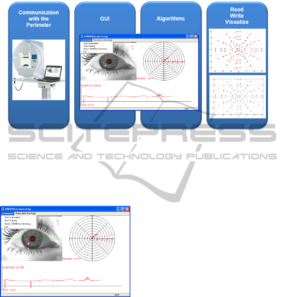
Figure 2: Components of the EFOV software.

for monitoring the eye position. In the future we

will use this information to monitor the vigilance

of the subjects during testing.

Furthermore the GUI provides several possibilities to

conﬁgure an examination, e.g. subject data, the set-

up of the stimulus grid, the size and duration of the

stimuli or the response time window.

Figure 3: The Graphical User Interface of EFOV. The left

upper part depicts the video signal from the cupola perime-

ter with the detected pupil (red circle). The presented stim-

ulus (black circle) and the gaze position of the subject over

the last 5 seconds are presented in a polar coordinate system

at the right upper part. The graph at the bottom depicts the

pupil size during the examination.

Read/Write and Visualization. A visualization ex-

ample of EFOV testing is presented in Figure 4(b).

The black dots indicate the presented stimuli (here the

stimuli grid consists of 72 stimuli locations in a po-

lar arrangement within the central 30

◦

ﬁeld of view).

The red dots represent the location of the subject’s

ﬁxations. Note that when a stimulus is presented, the

subject is asked to search for the presented stimulus

and then ﬁxate it. The presented stimulus (black dot)

and its corresponding ﬁxation point (red dot) are con-

nected by a red line. The longer the line, the greater

is the mismatch between presented stimulus and loca-

tion of the subject’s ﬁxation. Thus the length of the

line represents both the exploration quality and indi-

cates an overshoot or undershoot of the exploratory

saccade.

2.1 Algorithms

To be able to detect a ﬁxation during a video se-

quence, ﬁrst the gaze position of the subject at each

time step, i.e. video frame, has to be determined. The

gaze position is the position of the pupil midpoint in

the scene, i.e. cupola surface. For the detection of the

pupil and gaze position we perform image processing

of the video signal captured by the camera interface

in the Octopus perimeters. Furthermore, changes of

pupil size are monitored.

Pupil Detection. Real-time performance is a major

prerequisite to the image processing algorithms. We

use both global and local image features to extract

the pupil. The basic idea behind it is simple: since

the pupil represents an extended circular object with

dark pixels, we have to search for and ﬁnd such pixel

groups. First, global image properties, such as the av-

erage image brightness b

avg

, are calculated. Then, for

performance reasons, every second pixel is processed.

Its gray level value is compared to a threshold gray

ANewMethodforAssessingtheExploratoryFieldofView(EFOV)

level th that varies with the average image brightness.

This threshold is deﬁned as

th = α ∗b

avg

The variable α is set empirically and can be adjusted

by the user until the pupil detection is satisfactory.

Since other regions in the image, such as eye lashes,

may also contain dark pixel groups, for each detected

group of dark pixels, it is necessary to calculate the

brightness of its neighboring pixels. Only those pix-

els that are surrounded by dark pixels within a user-

deﬁned neighborhood area will be considered as can-

didates for the pupil. The pixel group that corre-

sponds to the pupil is found by shape matching as the

pixels corresponding to the pupil should form a cir-

cular object. Finally, for the identiﬁed pupil region,

the area and radius is calculated. We track the posi-

tion of the pupil center, which moves linearly with the

direction of gaze.

Gaze Mapping and Fixation Detection. To be able

to calculate the gaze position in the scene (i.e. on

perimeter surface), we need to provide a mapping be-

tween the position of the eye within the camera image

and the coordinates on the perimeter surface. The co-

ordinates of the eye position are deﬁned by the coor-

dinates of the pupil center. The mapping is calculated

during a calibration routine, as usual in eye-tracking

applications. We use a 3 × 3 calibration grid as pre-

sented by (Li et al., 2005).

The scene points

= (x

) are given in polar

coordinates and can be conﬁgured at the beginning

of an examination. We deﬁne following default val-

ues for the coordinates x

∈ {−20,0,20}. The re-

sulting nine points from the combination of these co-

ordinates are presented during the calibration routine

sequentially, where each point is presented for 5 sec-

onds (corresponding to 100 frames at the sampling

frequency of the camera). The subject is asked to ﬁx-

ate each presented calibration point. During stimulus

presentation the eye position ~e

= (x

) in the im-

age is calculated using the algorithms for the pupil

detection described above. When the eye position is

stable for a time period f

, a ﬁxation is assumed. In

order to achieve best mapping precision, during the

calibration procedure we expect long ﬁxations f

1000ms (corresponding to 20 video frames). Thus,

the standard deviation f

of the eye position in the im-

age data is computed for the last 20 frames. When the

standard deviation respects an empirically determined

threshold th

= 4px that considers the inaccuracy of

the eye tracker, f

< th

a ﬁxation is assumed. If a

ﬁxation cannot be recognized (e.g. due to an impaired

cooperation) the missed stimulus is presented again.

The mapping of the eye position in the image to

the gaze position in the scene, - perimeter surface - we

use a ﬁrst-order linear mapping (Li et al., 2005). For

each correspondence between

and ~e

, two equations

are generated that constrain the following mapping:

= a

+ a

= a

+ a

where a

and a

are undetermined coefﬁcients of

the linear mapping. This linear formulation results

in six coefﬁcients that need to be determined. Given

the nine point correspondences from the calibration

and the resulting 18 constraint equations, the coefﬁ-

cients can be solved using Single Value Decomposi-

tion (Hartley and Zisserman, 2000).

In a further step, for each presented stimulus

during the EFOV test, we have to ﬁnd out whether

the stimulus was ﬁxated by the subject. Generally,

when a presented stimulus is ﬁxated, the subject’s

gaze oscillates around the stimulus location forming

a ﬁxation cluster. A ﬁxation is assumed if the gaze

is kept around the stimulus location for at least 300

ms (Liversedge et al., 2011). At a sampling rate of

20 Hz, as it is the case in the built-in cameras of the

Octopus perimeter, 300ms correspond to 6 frames (or

gaze points). After the presentation of a stimulus, our

algorithm searches for clusters of points in at least

6 sequential video frame. This parameter is conﬁg-

urable and can easily be adapted to other sampling

rates. If a ﬁxation cluster is detected, we calculate

the cluster centroid that represents the location of

the ﬁxation. As described above, for each stimulus

location (Figure 4(b) black dots) we calculate the

corresponding ﬁxation location (Figure 4(b) red dots).

2.2 Modeling Fixation Data with the

Generalized Pareto Distribution

We observed that an exact match between the location

of the presented stimulus and the corresponding ﬁxa-

tion is given very rarely. Instead, for a given stimulus

location, the distribution of the distances between the

stimulus location and the ﬁxations of different sub-

jects corresponds to a Pareto distribution. The ques-

tion is: up to which distance between ﬁxation and

stimulus d

seen

can a stimulus be considered as per-

ceived (seen)?

We used the Generalized Pareto Distribution

(GPD) to model the distribution of distances between

ﬁxation and stimulus and implemented the model us-

ing Matlab (MATLAB, 2012). The probability den-

sity function of GPD is given by the following Equa-

tion 1 (Kotz and Nadarajah, 2000), (Embrechts et al.,

HEALTHINF2013-InternationalConferenceonHealthInformatics

1997):

y = f (d|k, σ, θ) = (

)(1 + k

(d − θ)

)

−1−

(1)

where d is the distance between stimulus location

and ﬁxation location, k 6= 0 is the shape parameter,

σ the scale parameter and θ the threshold parameter.

The threshold value d

seen

was obtained from the 95%

quantile of ﬁxations of healthy (control) subjects, see

Section 3.

3 RESULTS

EFOV was validated in a pilot study with 80 sub-

jects, 40 patients with binocular visual ﬁeld defects

and 40 ophthalmologically healthy (control) subjects.

The aim of the study was to investigate the prediction

capability of EFOV for everyday living conspicuous

objects within the central 30

◦

of the visual ﬁeld. Fur-

thermore, the driving performance of the subjects was

assessed in an on-road study using a dual-brake vehi-

cle. The scope of the study was much broader and

involved the investigation of visual scanning behavior

and its impact on the driving performance. The oph-

thalmological interpretation of the results of the study

is beyond the scope of this paper and will be presented

in a separate article. In the following we will focus on

some exemplary results of the assessment of the ex-

tended ﬁeld of view to show the viability of the soft-

ware.

To determine the threshold d

seen

, i.e. the maximal

distance between a perceived stimulus and the corre-

sponding ﬁxation, we ﬁtted the GPD model presented

in Equation 1 to the ﬁxation data collected from the

control subjects. From the 95% quantile we obtained

the threshold value d

seen

= 10. Thus, a stimulus is

considered as perceived, if the distance between its

location and the location of the corresponding ﬁxa-

tion does not exceed 10

◦

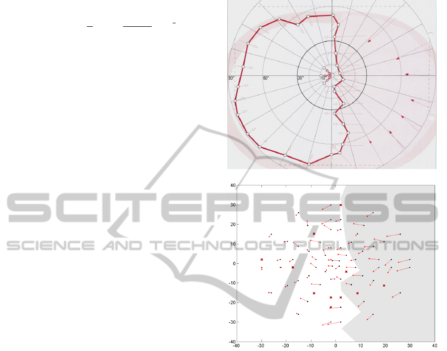
Figure 4(a) shows the binocular visual ﬁeld of a

subject with a homonymous visual ﬁeld defect that

was tested with semi-automated kinetic perimetry.

The red line represents the boundary of the intact vi-

sual ﬁeld. This subject is suffering from right-sided

hemianopsia, therefore he has no perception within

the right hemiﬁeld. Based on this result, the sub-

ject was banned from driving. Figure 4(b) depicts the

EFOV testing result. The gray area represents the vi-

sual ﬁeld defect from 4(a). The black dots represent

the locations of the presented stimuli, while the lo-

cations of the ﬁxation clusters are represented by red

dots. As mentioned above, the location of a stimu-

lus and its corresponding ﬁxation are connected by a

(a)

(b)

Figure 4: The performance of a subject with good ex-

ploration capability. The upper ﬁgure shows the result of

a standard semi-automated kinetic perimetric examination,

where the red line represents the boundary of the intact vi-

sual ﬁeld. The subject can perceive only stimuli that are

presented within the left hemiﬁeld. The lower ﬁgure shows

the result of the exploratory ﬁeld of view testing. The black

dots represent the locations of the presented stimuli. The

red dots are the locations of the subject’s ﬁxation. When eye

movements are allowed, this subject can obviously compen-

sate for his visual ﬁeld defect.

red line. Implicitly, the line length represents the ex-

ploration capability of a subject. The longer the line,

the greater is the mismatch between presented stimu-

lus and ﬁxation location. If the distance between the

location of a presented stimulus and the location of

the ﬁxation exceeds 10

◦

, the stimulus is considered

as not seen. Such ’failed-to-see’ stimuli and missing

ﬁxations (i.e. when no ﬁxation was detected within

a given response time window) are represented by

red crosses. As we can see from the distances be-

tween the stimuli locations and the locations of the

ANewMethodforAssessingtheExploratoryFieldofView(EFOV)

ﬁxations clusters, this patient has developed a good

visual search strategy that enables him to compensate

for his visual ﬁeld defect.

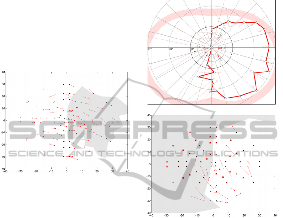
Another example for a successful visual search

strategy is shown in Figure 5. This subject can fully

compensate for his visual ﬁeld defect and is able to

perceive all stimuli presented in the area of his visual

ﬁeld defect. Interestingly, both subjects passed the

on-road driving assessment.

Figure 5: The EFOV result of a subject with a successful

visual search strategy.

Figure 6(a) presents the visual ﬁeld of another

subject suffering from left sided homonymous hemi-

anopsia. The lengths of the mismatch lines within the

right hemiﬁeld and the missed stimuli indicate poor

exploration capability. This subject failed the on-road

driving task.

4 CONCLUSIONS

In this paper we have presented a software for the as-

sessment of the exploratory ﬁeld of view using a con-

ventional cupola perimeter. Pilot studies conducted

so far have shown that this approach allows the as-

sessment of exploratory capabilities, which may be

more relevant than the extent and location of the vi-

sual ﬁeld defect. In contrast to standard perimetric

examinations, the assessment of EFOV promises to

reveal the the real impact of visual ﬁeld defects on ac-

tivities of daily living, such as driving. Yet, broader

evaluation of the method is needed.

Due to its modular structure, the EFOV software

can easily be extended by further modules. Our future

work will be threefold. As many subjects report loss

of vigilance during visual ﬁeld examinations, lead-

ing thus to an increase in the frequency of missed

(a)

(b)

Figure 6: The performance of a subject with left sided hemi-

anopsia. The upper ﬁgure shows the result of a standard

semi-automated kinetic perimetric examination. The lower

ﬁgure shows the result of the EFOV assessment. In contrast

to the results of the subjects in Figures 4(b) and 5, this sub-

ject could perceive only few of the stimuli within the visual

defect area. This indicates poor exploration capability.

targets, we will develop a module for the monitor-

ing of vigilance by using the pupillographic informa-

tion (Henson and Emuh, 2010). Furthermore we plan

the improvement of the calculation of ﬁxation clus-

ters using a Bayesian online clustering method (Tafaj

et al., 2012). Up to now EFOV was developed for

usage with Octopus perimeters. To make it available

for a broader set of applications, we plan to integrate

the testing method with existing vision analysis tools,

such as Vishnoo (Tafaj et al., 2011).

HEALTHINF2013-InternationalConferenceonHealthInformatics

REFERENCES

Embrechts, P., Kl

uppelberg, C., and Mikosch, T. (1997).

Modelling Extremal Events for Insurance and Fi-

nance. Springer.

Hardiess, G., Papageorgiou, E., Schiefer, U., and Mallot,

H. A. (2010). Functional compensation of visual ﬁeld

deﬁcits in hemianopic patients under the inﬂuence of

different task demands. Vision Res, 50(12):1158–

1172.

Hartley, R. and Zisserman, A. (2000). Multiple view geom-

etry in computer vision. Cambridge University Press,

Cambridge, UK.

Henson, D. and Emuh, T. (2010). Monitoring vigilance dur-

ing perimetry by using pupillography. Invest Ophthal-

mol Vis Sci, 51(7):3540–3543.

Kotz, S. and Nadarajah, S. (2000). Extreme Value Distri-

butions: Theory and Applications. Imperial College

Press, 1st edition.

Li, D., Winﬁeld, D., and Parkhurst, D. J. (2005). Starburst:

A hybrid algorithm for video-based eye tracking com-

bining feature-based and model-based approaches. In

Proceedings of the 2005 IEEE Computer Society Con-

ference on Computer Vision and Pattern Recognition

(CVPR’05), pages 1–8.

Liversedge, S., Gilchrist, I. D., and Everling, S. (2011). The

Oxford Handbook of Eye Movements. Oxford Univer-

sity Press.

Martin, T., Riley, M., Kelly, K. N., Hayhoe, M., and Huxlin,

K. R. (2007). Visually guided behavior of homony-

mous hemianopes in a naturalistic task. Vision Res,

47:3434–3446.

MATLAB (2012). version 7.14.0.739 (R2012a). The Math-

Works Inc., Natick, Massachusetts.

Pambakian, A. L., Wooding, D. S., Patel, N., Morland,

A. B., Kennard, C., and Mannan, S. K. (2000).

Scanning the visual world: a study of patients with

homonymous hemianopia. J Neurol Neurosurg Psy-

chiatry, 69:751–759.

Riley, M., Kelly, K. N., Martin, T., Hayhoe, M., and Huxlin,

K. R. (2007). Homonymous hemianopia alters distri-

bution of visual ﬁxations in 3-dimensional visual en-

vironments. J Vision, 7:289.

Schiefer, U., Wilhelm, H., and Hart, W. (2008). Clinical

Neuro-Ophthalmology: A Practical Guide. Springer

Verlag.

Tafaj, E., Kasneci, G., Rosenstiel, W., and Bogdan, M.

(2012). Bayesian online clustering of eye movement

data. In Proceedings of the Symposium on Eye Track-

ing Research and Applications, ETRA ’12, pages

285–288, New York, NY, USA. ACM.

Tafaj, E., K

ubler, T., Peter, J., Schiefer, U., Bogdan, M., and

Rosenstiel, W. (2011). Vishnoo - An Open-Source

Software for Vision Research. In Proceedings of

the 24

IEEE International Symposium on Computer-

Based Medical Systems, pages 1–6.

Taylor, J. F. (1982). Vision and driving. Practitioner,

226:885–889.

ANewMethodforAssessingtheExploratoryFieldofView(EFOV)