Grid-based Spatial Keypoint Selection for Real Time Visual Odometry

Volker Nannen

1∗

and Gabriel Oliver

2†

Departament d’Arquitectura i Tecnologia de Computadors, Universitat de Girona, Girona, Spain

Departament de Ci`encies Matem`atiques i Inform`atica, Universitat de les Illes Balears, Palma de Mallorca, Spain

Keywords:

Robot Vision, Robot Navigation, Real-time Systems, Robust Estimation, Spatial Distribution.

Abstract:

Robotic systems can achieve real-time visual odometry by extracting a ﬁxed number of invariant keypoints

from the current camera frame, matching them against keypoints from a previous frame, and calculating

camera motion from matching pairs. If keypoints are selected by response only they can become concentrated

in a small image region. This decreases the chance for keypoints to match between images and increases the

chance for a degenerate set of matching keypoints. Here we present and evaluate a simple grid-based method

that forces extracted keypoints to follow an even spatial distribution. The beneﬁts of this approach depend

on image quality. Real world trials with low quality images show that the method can extend the length of

a correctly estimated path by an order of magnitude. In laboratory trials with images of higher quality we

observe that the quality of motion estimates can degrade signiﬁcantly, in particular if the number of extracted

keypoints is low. This negative effect can be minimized by using a large number of grid cells.

1 INTRODUCTION

Precise real-time odometry is an active research ﬁeld

in underwater robotics. Autonomous underwater ve-

hicles usually rely on acoustic baseline stations and/or

dead reckoning for global localization. When operat-

ing close to the ground or to equipment that needs in-

spection and manipulation, visual odometry provides

a high level of precision at a relatively low cost. Mo-

tion can be estimated from a series of camera frames

by tracking a set of images features or keypoints that

are invariant under various image transformations.

After a ﬁrst processing step, a camera frame will of-

ten yield thousands of potential keypoints, each with

a response value (e.g., contrast) that is speciﬁc to the

feature detection method. Because of the computa-

tional cost involved in constructing an invariant key-

point descriptor and matching it against another set

of keypoint descriptors, from the initially large num-

ber of m keypoints only those n ≪ m keypoints with

the highest response value will be extracted, as those

are most likely to be detected in another image of the

same scene. A threshold response value is often used,

∗

Supported by the Spanish Ministry of Education and

Science’s Juan de la Cierva contract JCI-2011-10400.

†

Supported by the European Commission’s Seventh

Framework Programme FP7/2007-2013 under grant agree-

ment 248497 (TRIDENT Project).

but in real time odometry it is more convenient to se-

lect a ﬁxed number of keypoints with the highest re-

sponse, say 100 (Nannen and Oliver, 2012).

Underwater, satisfactory visibility often requires a

distance of no more than one or two meters from the

inspected surface. Objects fade with distance, which

makes the clarity of detail highly variable on irregular

surfaces. Even on ﬂat surfaces we ﬁnd that regions

which are rich in features often alternate with regions

that are virtually featureless. Feature rich objects like

crustaceans tend to concentrate the high response key-

points in small image regions. As a result, the set

of extracted keypoints might not overlap between im-

ages, or, if keypoints overlap and match, they might

come from too small a region to allow for a reliable

motion estimate with six degrees of freedom. A small

feature rich object like a crustacean might also have

its own independent trajectory.

An obvious remedy is to force the extracted key-

points to follow a more or less even spatial distribu-

tion over the image. In practice this means that se-

lection by response needs to be interwoven with se-

lection by spatial density. The literature provides a

number solutions that offer promising results. (Brown

et al., 2005) introduced adaptive non-maximal sup-

pression (ANMS) to achieve such an even distribu-

tion. This method calculates for each keypoint a sup-

pression radius, which is the distance to the closest

586

Nannen V. and Oliver G. (2013).

Grid-based Spatial Keypoint Selection for Real Time Visual Odometry.

In Proceedings of the 2nd International Conference on Pattern Recognition Applications and Methods, pages 586-589

DOI: 10.5220/0004270005860589

 SciTePress

keypoint with signiﬁcantly higher response, and se-

lects the keypoints with the largest suppression ra-

dius for further processing. ANMS reports promis-

ing results but suffers from quadratic time complex-

ity in the number of considered keypoints. (Gauglitz

et al., 2011) suggest a number of heuristics to reduce

the time complexity of ANMS, and also offer an im-

proved version of ANMS, called suppression via disk

covering, which is of time complexity O(mlogm).

By contrast, (Cheng et al., 2007) achieve an even

spatial distribution by distributing keypoints over a

given number of c cells by means of a k-d tree. Start-

ing with a cell that covers the entire image and con-

tains all keypoints, the algorithm divides the cells re-

cursively into smaller cells, each containing half the

keypoints of the mother cell. For each division, the

spatial variance along the x and y-axis is computed,

and the cell is divided along the median value of the

dimension that has the larger variance. From the key-

points of each cell the n/c keypoints with the highest

response value are then selected for further process-

ing, again achieving a time complexity of O(mlogm).

(Cheng et al., 2007) recommend c = 64 cells if n =

100 keypoints are to be extracted.

Here we study and evaluate a selection method

that is even simpler than even k-d trees. We propose

to partition an image into a regular grid of c cells, to

assign all detected keypoints to their corresponding

cells, and to select from each cell the n/c keypoints

with the highest response value. As sorting by re-

sponse value cannot be avoided, the time complexity

is again O (mlogm), yet the constant factor is reduced

to a minimum. That is, compared with k-d trees, we

eliminate the need to calculate the variance in x and y-

dimension and the median for the winning dimension

for m keypoints for every division level. Calculation

of the median requires an extra sort at every division

level. K-d trees with 64 cells requires log

64 = 6 di-

vision levels and 7 sorts, while grid-based selection

requires only one sort.

Real world trials on underwater images show that

already a 2x2 grid can lead to dramatic improvement

over selection by response only. A 2x2 grid requires

only two greater-than comparison operations per key-

point, yet in our trials it extended the average vehicle

distance over which the visual odometer can correctly

estimate motion by an order of magnitude, from sev-

eral meters to several dozens of meters. The images

of these trials were recorded by remote vehicle off the

coast of the Balearic island of Mallorca and contain

thousands of images per sequence. The vehicle op-

erator tried to steer the vehicle at an average distance

of 1 meter from the sea ﬂoor. Due to the rocky na-

ture of the underwater terrain, with frequent boulders,

cliffs, and crevices, actual distance to image objects is

highly variable, as is the clarity of image features be-

tween images. It is important to note that in this case,

doubling the number of extracted keypoints per im-

age did not signiﬁcantly increase the average length

of correct motion estimates.

Visual inspection of image pairs for which a 2x2

grid gave such a dramatic improvement shows that

they are typically of low quality—bad lighting and

much blur and fade—over most of the image, but

with a small image region of medium quality, such

that almost all extracted keypoints cover that small

region. This small region is then either not present

in both images of a pair, or has changed signiﬁcantly

between images due to changes in lighting, blur or

fade. Response-based selection continues to be con-

centrated on this small region even when more key-

points are extracted, while grid-based selection forces

the low-quality region to be considered as well.

With this promising result at hand, the question

arises whether grid-based selection is also beneﬁcial

or at least not detrimental when motion can already

be estimated well with response-based selection only.

If it is detrimental, a real-time system might require

additional logic to decide when to use grid-based se-

lection and when not. In the remainder of this article

we report on systematic experiments in a highly con-

trolled environment that evaluate the effect of grid-

based selection on motion estimates from image se-

quences of higher quality than in the real-world trials

described above.

2 EXPERIMENTAL SETUP

We base our evaluation on over 2,000 images that

were collected by a downward looking camera aboard

the Girona500 autonomous submarine (Prats et al.,

2012) during two controlled test dives in the labora-

tory pool of the VICOROB research group in Girona.

Image resolution is 384 by 288 pixels. Lighting con-

ditions were good and the water was clean. Motion

blur and light scatter are negligible. The ﬂoor of the

pool was covered by a life-size high resolution color

poster that shows a coral reef off the coast of Florida.

The poster was spread out ﬂat, resulting in a planar

image scene. The digital version of the poster allows

us to calculate the ground truth per images with an ac-

curacy of 0.5 pixels. For a complete description of the

image acquisition and the calculation of the ground

truth see (Nannen and Oliver, 2012).

With a planar scene, motion can be estimated by

computing the homography that projects keypoints

from one image coordinate frame to the coordinate

Grid-basedSpatialKeypointSelectionforRealTimeVisualOdometry

587

frame of another image. A homography can be de-

composed into the rotation of the camera around its

axes, translation of the camera along the x and the y-

axis of the camera plane, and translation along its z

axis up to a scale parameter. See (Caballero et al.,

2009) for an overview of recent methodology. Roll

and pitch of the Girona500 did not exceed the ob-

served measurement error, and so we will consider

only yaw in the analysis.

For feature extraction and description we use

two independent open source implementations of the

SURF algorithm (Bay et al., 2008) without modiﬁ-

cation: one by (Evans, 2009) and one included in the

OpenCV image processing library which is developed

and distributed by Willow Garage. For reference we

also report results on the SIFT algorithm, again as

included in the OpenCV library. For the computa-

tion of the homography we use RANSAC (?, Ran-

dom Sample Consensus,)]Fischler:1981 in combina-

tion with least squares.

The Girona500 moved at a constant altitude of

one meter over the poster. Its path consisted of 10

stretches of either 2 or 4 meters length, with 18 right

angle turns in between. During the straight runs,

the robot occasionally slowed down, rotated to adjust

its path, and continued. We considered pairs of im-

ages that are consecutive (distance 1) and that are of

distance {2, 3,. .. , 30}, totalling over 60,000 image

pairs. Average motion between images is 10 pixels,

mostly along the vertical axis, such that 2 consecutive

images overlap by 96%, and images at distance 10

still overlap by 2/3 of their area. Images at distance

30 only overlap if the robot slowed down or turned.

We consider 17 different grid arrangements, from

a grid size of 1, which is the 0-hypothesis, to a grid

size of 5× 8 = 40 cells. We consider 3 different num-

bers n of extracted keypoints per image: 50, 100, and

200. For each grid arrangement and for each value of

n we try to calculate a motion estimate for all 60,000

image pairs. When the number of grid cells is not a

multiple of the number of extracted image keypoints,

for example 30 grid cells and 100 extracted keypoints,

we ﬁrst allocate a larger multiple of keypoints over

the grid cells, 120 in this example, so that every cell

has 4 keypoints. We then order all cells by the lowest

response value of the keypoints they contain, and re-

move the lowest keypoints from those cells that rank

lowest until the desired number of keypoints is ob-

tained. In this example, that would leave 10 cells with

4 keypoints, and 20 with 3 keypoints. Note that this

additional sort is over the number c of cells, not over

the much larger number m of keypoints.

When evaluating the quality of a motion estimate

we distinguish between the error in spatial translation,

Table 1: Deﬁnition of quality thresholds.

t.h. I

at least 6 inliers

t.h. II e

x,y

≤ 1.82 e

yaw

≤ .008 e

scale

≤ .021

t.h. III

x,y

≤ 0.75 e

yaw

≤ .004 e

scale

≤ .008

t.h. IV e

x,y

≤ 0.33 e

yaw

≤ .002 e

scale

≤ .003

the error in rotation about the z axis, and error in scale.

The translation error e

x,y

is the Euclidean distance in

pixels between the translation vector of the motion es-

timate that is based on the homography between two

images, and the translation vector according to the

ground truth. The rotation error e

yaw

is the absolute

difference in radians between yaw as measured from

the homographies between two images, and yaw ac-

cording to the ground truth. A homography allows

for the robot motion along the z axis of the camera to

be computed only up to scale. Since this scale varies

only slightly in this image set, always being close to

one, we will only consider an error in the estimation

of its real value. We deﬁne the scaling error e

scale

the absolute difference between the relative scale as

measured from the homography between two images

and the relative scale according to the ground truth.

To quantify the quality of a motion estimate we

count the number of image pairs that pass certain

quality thresholds. The lowest quality threshold,

threshold I, counts the number of image pairs with

at least six inliers as selected by RANSAC. Three

more thresholds count the number of image pairs

with translation, rotation and scaling errors that are

all lower than some respective predeﬁned error levels

x,y

, e

yaw

, and e

scale

. See (Nannen and Oliver, 2012)

for a discussion of the problem of suitable thresholds,

and the choice presented in Table 1.

3 RESULTS

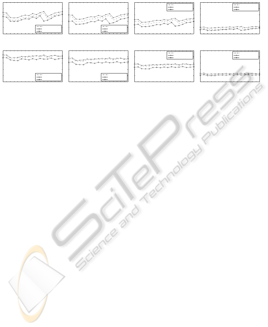
Figure 1 shows the results for 50 and 100 extracted

keypoints per image. Results for 200 extracted key-

points per image are very similar to those for 100 ex-

tracted keypoints, but lie 5 percent points higher on

the y-axis. The results are clear insofar as grid-based

spatial distribution never improves the estimate when

image quality is good, and signiﬁcantly degrades it

for low numbers of extracted keypoints and low num-

bers of grid cells. The worst performance can be ob-

served for 50 keypoints, 4 or 6 cells, in which case

the number of image pairs for which the motion es-

timate the given thresholds decreases by about 25%.

With larger numbers of grid cells the performance ap-

proaches that of no grid-based spatial distribution, but

never exceeds it.

ICPRAM2013-InternationalConferenceonPatternRecognitionApplicationsandMethods

588

REFERENCES

Bay, H., Ess, A., Tuytelaars, T., and van Gool, L. (2008).
Speeded-Up Robust Features (SURF). Computer Vis.
Image Underst., 110(3):346–359.
Brown, M., Szeliski, R., and Winder, S. (2005). Multi-
image matching using multi-scale oriented patches.
In IEEE Conf. Comput. Vision Pattern Recogn.,
CVPR’05, pages 510–517. IEEE.
Caballero, F., Merino, L., Ferruz, J., and Ollero, A. (2009).
Vision-Based Odometry and SLAM for Medium and
High Altitude Flying UAVs. J. Intell. Robotic Syst.,
54(1-3):137–161.
Cheng, Z., Devarajan, D., and Radke, R. J. (2007). De-
termining Vision Graphs for Distributed Camera Net-
works Using Feature Digests. EURASIP J. Adv. Signal
Process., 2007(1):057034.
Evans, C. (2009). Notes on the OpenSURF Library. Tech-
nical Report CSTR-09-001, University of Bristol.
Fischler, M. A. and Bolles, R. C. (1981). Random sample
consensus: a paradigm for model fitting with appli-
cations to image analysis and automated cartography.
Comm. ACM, 24(6):381–395.
Gauglitz, S., Foschini, L., Turk, M., and Hollerer, T. (2011).
Efficiently selecting spatially distributed keypoints for
visual tracking. In IEEE Int. Conf. Image Process.,
ICIP’11, pages 1869–1872. IEEE.
Nannen, V. and Oliver, G. (2012). Optimal Number of
Image Keypoints for Real Time Visual Odometry.
In IFAC Worksh. Navig. Guid. Control Underw. Veh.
(NGCUV), pages 1–6, Porto.
Prats, M., Ribas, D., Palomeras, N., Garc´ıa, J. C., Nannen,
V., Wirth, S., Fern´andez, J. J., Beltr´an, J. P., Cam-
pos, R., Ridao, P., Sanz, P. J., Oliver, G., Carreras, M.,
Gracias, N., Mar´ın, R., and Ortiz, A. (2012). Recon-
figurable AUV for intervention missions: a case study
on underwater object recovery. Intel. Serv. Robot.,