
Optimization of an Autostereoscopic Display for a Driving Simulator
Eva Eggeling
1
, Dieter W. Fellner
2,3
, Andreas Halm
1
and Torsten Ullrich
1
1
Fraunhofer Austria Research GmbH, Inffeldgasse 16c, Graz, Austria
2
Institute of Computer Graphics and Knowledge Visualization, TU Graz, Graz, Austria
3
GRIS, TU Darmstadt & Fraunhofer IGD, Darmstadt, Germany
Keywords:
Raster Display Devices, Virtual Reality, Global Optimization.
Abstract:
In this paper, we present an algorithm to optimize a 3D stereoscopic display based on parallax barriers for
a driving simulator. The main purpose of the simulator is to enable user studies in reproducible laboratory
conditions to test and evaluate driving assistance systems. The main idea of our optimization approach is to
determine by numerical analysis the best pattern for an autostereoscopic display with the best image separation
for each eye, integrated into a virtual reality environment.
Our implementation uses a differential evolution algorithm, which is a parallel, direct search method based
on evolution strategies, because it converges fast and is inherently parallel. This allows an execution on a
network of computers. The resulting algorithm allows optimizing the display and its corresponding pattern,
such that a single user in the simulator environment sees a stereoscopic image without being supported by
special eye-wear.
1 INTRODUCTION
The concept of a 3D display has a long and varied
history stretching back to the 3D stereo photographs
made in the late 19th century through 3D movies in
the 1950’s, holography in the 1960’s and 1970’s and
the 3D computer graphics and virtual reality of today
– as summarized by PHILIP BENZIE et al. in “A Sur-
vey of 3DTV Displays” (Benzie et al., 2007).
Taking all the options into account to realize a
3D-display (Lancelle, 2011), our customer chose a
parallax-barrier-based autostereoscopic display due
to its cost-efficiency. The field of application is a driv-
ing simulator, which shall be used to test and evalu-
ate driving assistance systems in user studies in re-
producible laboratory conditions; i.e. the main user
in this specialized virtual reality (VR) environment is
a driver in a typical driving position. This setting of-
fers the possibility to adopt the VR visualization with
extensive assumptions.
Therefore, we focus on the parallax barriers and
present a way to optimize it. Using numerical analy-
sis in combination with geometric modeling, we show
that it is possible to determine the best setup configu-
ration for a parallax barrier and to predict its quality,
in terms of separable pixel, even during the simula-
tor’s planning phase. This optimization approach is
beneficial not only for autostereoscopic displays but
for optimized VR-environments in general.
2 RELATED WORK
2.1 3D Displays & Parallax Barrier
A graphical display is termed autostereoscopic when
all of the work of stereo separation is done by the dis-
play (Eichenlaub, 1998), so that the observer does not
need to wear special eye-wear.
Nowadays, a wide range of autostereoscopic dis-
play technologies exists. While technologies like
holographic displays can still be considered experi-
mental, other technologies, like variations of parallax
barriers or lenticular lenses which have been utilized
by several consumer TVs as well as the Nintendo 3DS
handheld console, are already quite common (Benzie
et al., 2007).
These binocular display types are quite simple to
produce but have a number of limitations. The most
important one is, that they are limited to one user
whose position needs to be fixed or is at least lim-
ited to a few viewing spots. For the parallax barrier
method a fine vertical grating or lenticular lens ar-
318
Eggeling E., Fellner D., Halm A. and Ullrich T..
Optimization of an Autostereoscopic Display for a Driving Simulator.
DOI: 10.5220/0004290203180326
In Proceedings of the International Conference on Computer Graphics Theory and Applications and International Conference on Information
Visualization Theory and Applications (GRAPP-2013), pages 318-326
ISBN: 978-989-8565-46-4
Copyright
c
2013 SCITEPRESS (Science and Technology Publications, Lda.)

Figure 1: An autostereoscopic display can be realized us-
ing a parallax barrier. The barrier is located between the
eyes (visualized in blue and red) and the pixel array of the
display. It blocks certain pixels for each eye, which results
in the eyes seeing only disjoint pixel columns (at least in
an optimal setting). If the display is fed with correct image
data, the users sees a stereo image.
ray is placed in front of a display screen. If the ob-
server’s eyes remain fixed at a particular location in
space, then one eye can see only the even display pix-
els through the grating or lens array, and the other eye
can see only the odd display pixels (see Figure 1).
The limitation to a single user is not a problem in
this scenario since it is limited to one user (the driver)
anyway. The other major drawback of this approach,
namely the fact that the observer must remain in a
fixed position, can be lifted by virtually adjusting the
pixel columns such that the separation remains intact,
as presented in (Sandin et al., 2001; Peterka et al.,
2007). For this to work, some kind of user tracking is
needed which also limits the amount of possible users.
Since the user’s possible positions are very lim-
ited in this scenario, there is no need to adjust for
user movement other than head rotation. Especially,
there is no need to adjust for large distance variations,
for example, using a dynamic parallax barrier (Perlin
et al., 2000).
Most consumer products containing autostereo-
scopic displays, however, just combine parallax bar-
riers with lenticular lenses, which does not put any
constraints on the number of possible users at a time.
This approach is relatively restricted concerning the
possible viewing position(s).
The one remaining drawback of this technique is
that the resolution drops down to a half for just a sin-
gle user. In the presented scenario, this is not a critical
point since the available resolution is quite high.
2.2 Numerical Analysis
An optimization problem can be represented in the
following way: For a function f mapping elements
from a set A to the real numbers, an element x
0
∈A is
sought-after, such that
∀x ∈ A : f (x
0
) ≤ f (x). (1)
Such a formulation is called a minimization problem
and the element x
0
is called a global minimum. De-
pending on the field of application, f is called an ob-
jective function, cost function, or energy function. A
feasible solution that minimizes the objective function
is called the optimal solution.
Typically, A is some subset of the Euclidean space
R
n
, often specified by a set of constraints (equalities
or inequalities) that the elements of A have to fulfill.
Generally, a function f may have several local min-
ima, where a local minimum x
?
satisfies the expres-
sion f (x
?
) ≤ f (x) for all x ∈ A in a neighborhood of
x
?
. In other words, in some region around x
?
all func-
tion values are greater than or equal to the value at x
?
.
The occurrence of multiple extrema makes problem
solving in (nonlinear) optimization very hard. Usu-
ally, the global (best) minimizer is difficult to identify
because in most cases our knowledge of the objective
functional is only local and global information are not
available. Since there is no easy algebraic character-
ization of global optimality, global optimization is a
difficult area,especially in higher dimensions.
Further explanations on global optimization can
be found in “Numerical Methods” (Boehm and
Prautzsch, 1993), “Numerical Optimization” (No-
cedal and Wright, 1999), “Introduction to Applied
Optimization” (Diwekar, 2003), “Compact Numer-
ical Methods for Computers: Linear Algebra and
Function Minimisation” (Nash, 1990), as well as in
“Numerische Methoden der Analysis” (english: Nu-
merical Methods of Analysis) (H
¨
ollig et al., 2010).
Besides these introductions and overviews some
books emphasize practical aspects – e.g. “Practical
Optimization” (Gill et al., 1982), “Practical Methods
of Optimization” (Fletcher, 2000), and “Global Op-
timization: Software, Test Problems, and Applica-
tions” (Pinter, 2002).
All optimization algorithms can be classified in
gradient-based methods, which use the objective
function’s derivatives, and non-gradient-based meth-
ods, which do not rely on derivatives. As most gradi-
ent based methods optimize locally, they most likely
find local minima of a nonlinear function but not its
global minimum. To find a global minimum local
optimization algorithms can be combined with ge-
netic algorithms (Janikow and Michalewicz, 1990),
(Michalewicz, 1995), (Michalewicz and Schoenauer,
1996) which have good global search characteris-
tics (Okamoto et al., 1998). These combinatorial
methods – such as simulated annealing (Ingber, 1993)
– improve the search strategy through the introduction
of two tricks. The first is the so-called “Metropolis
algorithm” (Metropolis et al., 1953), in which some
iterations that do not lower the objective function are
accepted in order to “explore” more of the possible
space of solutions. The second trick limits these ex-
OptimizationofanAutostereoscopicDisplayforaDrivingSimulator
319
plorations, if the cost function declines only slowly.
Our implementation uses such an algorithm: dif-
ferential evolution (Storn and Price, 1997). It is a par-
allel, direct search method based on ideas of evolution
strategies. It uses n vectors x
i,k
(i = 1,...,n) as a pop-
ulation for each generation k. The members of a new
generation k + 1 are generated by a permutation and a
cross-over process. For each vector x
i,k
a trial vector
∆ = x
α,k
+ F ·(x
β,k
−x
γ,k
) (2)
is generated with a constant F ∈ R, F > 0, and ran-
domly chosen α,β,γ ∈ {1,...,n}\{i}, which do not
equal each other α 6= β 6= γ 6= α.
To increase the diversity of the parameter vectors,
a cross-over process mixes x
i,k
with ∆. The result-
ing vector y consists of a sequence of elements of
x
i,k
, whereas other elements are copied from ∆. If
the new vector y yields a smaller objective function
value than x
i,k
, then x
i,k+1
is replaced by y otherwise
the old value x
i,k
is retained.
The differential evolution method for minimizing
continuous space functions can also handle discrete
problems by embedding the discrete parameter do-
main in a continuous domain. It converges quite fast
and is inherently parallel, which allows an execution
on a network of computers.
3 ALGORITHMIC OVERVIEW
The main idea of our optimization approach is to de-
termine the best pattern for an autostereoscopic dis-
play by numerical analysis; i.e. the pattern (as illus-
trated in Figure 1) has free parameters (line width,
line distance, and line orientation) and is interpreted
as a function. Embedded into a geometric scene the
objective function simply counts the number of pix-
els, which can be seen by both eyes, or which cannot
be seen at all. If this value is minimized, the number
of pixel, which can be seen only by one eye is maxi-
mized. As a consequence, the best image separation
is reached.
3.1 Geometric Description
In detail, the objective function is an algorithmic rou-
tine, whose inner structure is very similar to a ray
tracer. It consists of the components display, pattern,
occluder and eyes, as described below:
Display. The display, respectively its 2D pixel array,
is defined by its four corner points in R
3
, which
form a planar rectangle, and its horizontal h and
vertical w resolution. These parameters are fixed
and not subject to the optimization.
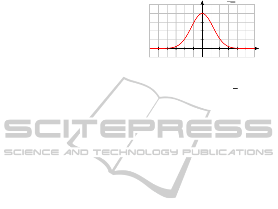
t
f (x) =
1
√
2π
e
−x
2
/2
1
/
2
0 4−4
Figure 2: A random variable X has a Gaussian distribution
with mean µ and variance σ
2
; written X ∼N(µ,σ
2
), if it has
a probability density function f (x) =
1
σ
√
2π
e
−(x−µ)
2
/(2·σ
2
)
.
This plot shows the standard normal distribution N(0,1).
Based on this display definition a sequence of pix-
els
P = {p
1
,p
2
,...,p
h×w
} (3)
in 3D is generated.
Pattern. The parallax barrier is defined by seven pa-
rameters. Four of them are points in 3D space,
which form a planar rectangle, and three values
describe the pattern itself (the line width l
w
, the
distance between two consecutive lines l
d
mea-
sured between medial axes, and their deviation
from a vertical alignment l
α
). These three vari-
ables
(l
w
,l
d
,l
α
) (4)
are subject to the optimization.
Occluder. The geometric description also contains
occluders – simple triangles, which are used to de-
scribe, e.g., the car’s geometry in Section 5.
Eyes. The eyes are specified by a center point, a look-
at-direction and an up-direction, which define a
local coordinate system. Together with the eye-to-
eye distance the position of the left and the right
eye are calculated.
Similar to light sampling approaches, in ray trac-
ing we sample the eyes in order to describe area
lights by point lights. Ten parameters describe the
average eye movement; i.e. the center position
(in all, three coordinate axes) as well as the look-
at-direction (respectively its angular components
of spherical coordinates) are weighted and spread
according to stochastically independent Gaussian
distributions specified by mean and variance for
each coordinate component (see Figure 2). Based
on this description a stochastic sampling is per-
formed, which results in a list of eye positions
E = {(e
L
,e
R
)
1
,(e
L
,e
R
)
2
,...,(e
L
,e
R
)
m
}. (5)
GRAPP2013-InternationalConferenceonComputerGraphicsTheoryandApplications
320

3.2 Objective Function
Depending on the free parameters (l
w
,l
d
,l
α
), a ge-
ometric scene is created, which results in a classifi-
cation of pixels (for this particular setting) as shown
in Figure 3: each pixel is seen by both eyes (illus-
trated in white), by one eye only (red or blue), or by
no eye (black). The objective function simply counts
the number of pixels, which can be seen by both eyes,
or which cannot be seen at all.
In detail, the objective function is
f (l
w
,l
d
,l
α
) =
∑
p∈P
∑
(e
L
,e
R
)∈E
isVisible
occ∪pattern(l
w
,l
d
,l
α
)
(e
L
,p) XNOR
isVisible
occ∪pattern(l
w
,l
d
,l
α
)
(e
R
,p)
,
(6)
where occ ∪ pattern(l
w
,l
d
,l
α
) is a list of geometric
occluders, which comprehends static occluders occ,
such as a car’s geometry, and dynamic occluders, i.e.
the parallax barrier pattern defined by (l
w
,l
d
,l
α
).
As the objective function iterates over all pixels
and calculates a “small” result – one whose size does
not depend on the input data set and therefore is con-
stant – it is implemented using the estimation tech-
nique presented in “Linear Algorithms in Sublinear
Time” (Ullrich and Fellner, 2011). This technique re-
duces the needed time for a display optimization to a
few minutes each.
The optimization routine has been tested for two
settings: a simple desktop environment with a single
display and the simulator environment with 24 dis-
plays. As the optimization process is the same for
both environments, we only describe the desktop en-
vironment in detail. For the simulator environment
only the differences are outlined.
Figure 3: In a parallax barrier setting all pixels can be clas-
sified according to their visibility. Pixel can either be seen
by both eyes (visualized in white), by one eye only (red or
blue), or by no eye (black). Depending on the eyes’, the
display’s and the barrier’s position in 3D a characteristic
pattern comes into existence. As an ideal pattern does not
contain any black or white pixels, the optimization routine
optimizes the pattern for stochastically sampled eye posi-
tions and minimizes the sum of black and white pixels.
4 DESKTOP SETTING
4.1 Geometric Measurement
In order to arrange the display and the parallax bar-
rier properly, the metrics of the monitor is needed –
especially the distance between the pixel array inside
the LCD and the outer surface of the glass panel. As
this value is normally not documented by the manu-
facturer and as we do not want to void the hardware-
guarantee terms, we used a 3D laser scanner to mea-
sure the desired distance. Figure 4 shows the scan-
ning process. With a Post-it note on the glass pane,
the scanner returns a triangular mesh of the Post-it as
well as a few more triangles from inside the monitor.
Figure 4: A laser scanner can be used to measure the dis-
tance between the outer surface of the glass pane and the
pixel array inside without having to open the display and
violating the hardware guarantee terms.
The result of the scanning process is visualized in
Figure 5. It shows the Post-it’s geometry (in yellow)
and a plane fitted to it (in blue). The fitted plane is
used as a reference for the outer surface of the glass
pane. The “few more triangles” also found in the data
set correspond to the inner pixel array. Another plane,
fitted exclusively to these triangles, is also shown in
Figure 5 (in red). The distance between these planes
reveals a distance between the outer surface and the
Figure 5: The scan towards the inside of a display (see
Figure 4) reveals geometric measurements normally not
documented by manufacturers; e.g. the distance between
the outer surface (on which a sticky note has been placed,
shown in yellow and approximated by the blue plane) and
the inner pixel array (approximated by the red plane).
OptimizationofanAutostereoscopicDisplayforaDrivingSimulator
321
10.0mm
0.0mm
2.5mm
5.0mm
7.5mm
10.0mm
0.0mm
2.5mm
5.0mm
7.5mm
+20.0°
-20.0°
-10.0°
0.0°
+10.0°
100.0%
0.0%
25.0%
50.0%
75.0%
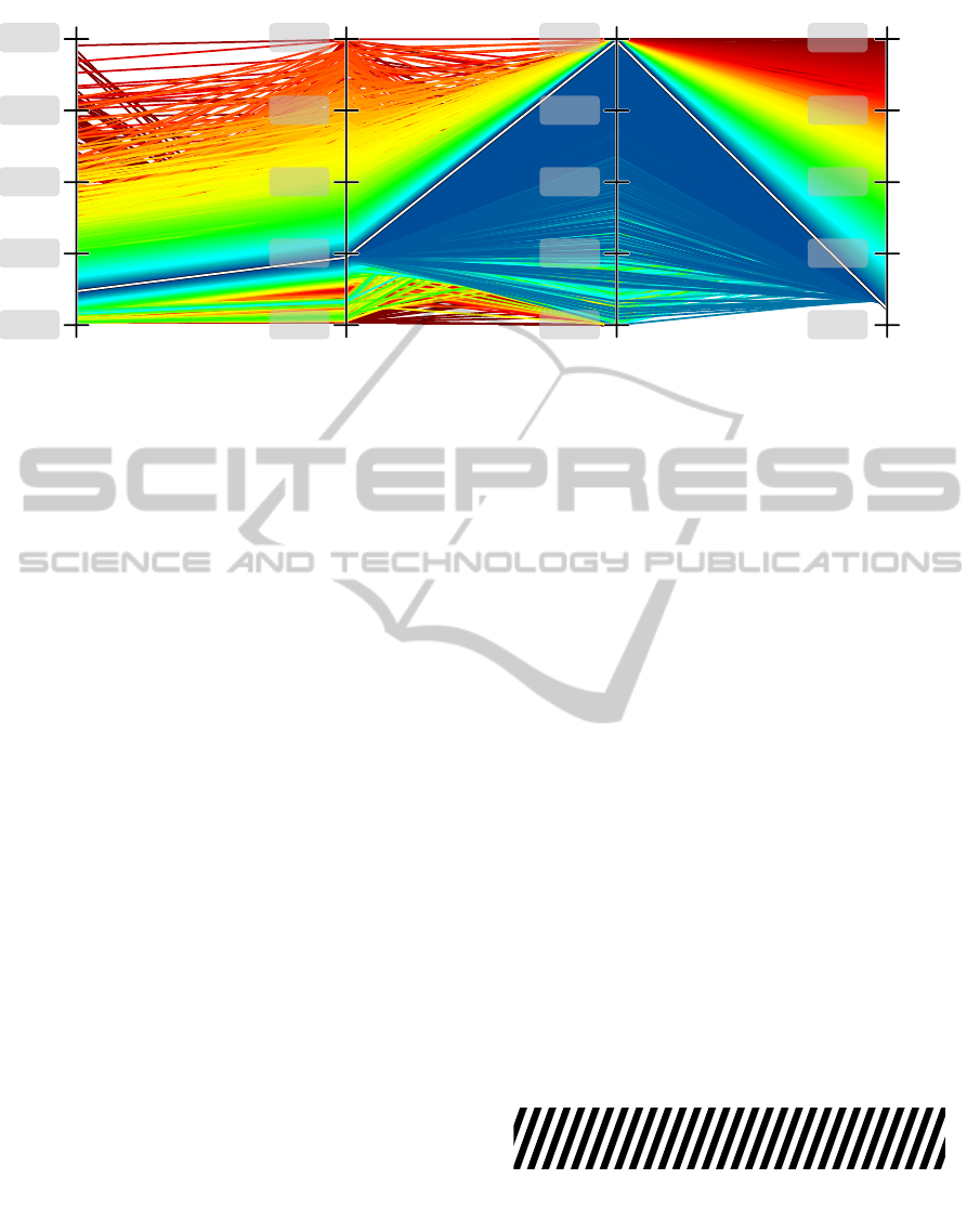
line width line distance line orientation non-separable
pixels
Figure 6: All evaluations of the objective function are plotted in parallel coordinates – a common way of visualizing multi-
variate data. Each objective function call is represented by a polyline, connecting its input parameters (“line width” on first
axis, “line distance” on second axis, and “line orientation” on third axis) with its function value (“non-separable pixels” on
last axis). In order to emphasize the minimization result, the polylines are hue color-coded and sorted from back (worst pa-
rameter) to front (best parameter). While the best “width” and “distance” parameters can be identified easily, the “orientation”
parameter has only limited influence on the objective function. This leads to a wide interval of good values along the “line
orientation” axis.
inner pixel array of 5.1mm for the iMac shown in Fig-
ure 4. The other geometric values (display position in
3D, user position in 3D) have been measured easily.
Furthermore, user’s eyes’ movement approximated by
a normal distribution has been estimated roughly.
4.2 Parallax Barrier Optimization
Having set the geometric input parameters, the opti-
mization routine determined the best solution within
the parameter domain
[0.1mm,0.1mm,−20
◦
] −[10.0mm, 10.0mm, +20
◦
];
(7)
i.e. the minimum line width and distance is 0.1mm,
the maximum line width and distance is 10.0mm,
and the line orientation may vary between −20
◦
and
+20
◦
. All evaluations of the objective function are
plotted in Figure 6 using parallel coordinates (Insel-
berg, 2009). Each objective function call is plotted as
a polyline, connecting its parameters with its function
value (axes from left to right: input parameters “line
width”, “line distance”, “line orientation”, and result-
ing “non-separable pixels”). In order to emphasize the
minimization result, the polylines are hue color-coded
and sorted from back (worst parameter) to front (best
parameter). Furthermore, the optimal result
1.1828mm 2.3651mm 19.7
◦
(8)
is highlighted.
This parameter setting results in a configuration,
in which 5.7288% of all pixels cannot be seen by one
eye only. Although the objective function has no reg-
ulation terms to ensure the balance between the num-
ber of pixels seen by the left eye in comparison to the
number of pixels seen by the right eye, the optimal
result is balanced.
In order to analyze the importance of the “line
orientation” parameter additional function evalua-
tions have been added. Especially the parameter set
(
1.1828mm 2.3651mm 0
◦
) has been tested and
returned a slightly higher and therefore non-optimal
value of 6.7946% non-separable pixels. Nevertheless,
the “line orientation” parameter is not very important:
configurations similar good as the optimal one can be
found along the complete “line orientation” axis in
Figure 6.
The resulting pattern of the globally optimal con-
figuration is shown in Figure 7 (in 1:1 original size).
In order to avoid local minima, the result has been
checked using the “Probability of Globality” tech-
nique (Eggeling et al., 2013).
Figure 7: For the desktop setting described in Section 4,
the optimal parallax barrier has lines, which are 1.1828mm
thick. The lines have a distance of 2.3651mm to each other
(measured from medial axis to medial axis) and are rotated
by 19.7
◦
.
GRAPP2013-InternationalConferenceonComputerGraphicsTheoryandApplications
322

5 SIMULATOR SETTING
5.1 Geometric Arrangement
The major goal of the manual arrangement procedure
was to block the driver’s view as good as possible;
i.e. from the driving position it should not be possible
to see the real environment. Only the virtual envi-
ronment, that is shown on displays, should be visible.
The most important part of the view is the windscreen,
while the side windows play only a minor role. There-
fore, 20 of the available 24 monitors are aligned in
front of the car, while two monitors are reserved for
each side.
For the process of optimizing the layout the mod-
eling and ray tracing software blender (Blain, 2012)
has been used. A model of the car was centered in
the scene, surrounded by a cylinder. A perspective
camera was put between the eye positions and was set
up to create a 180
◦
horizontal, 90
◦
vertical panoramic
image (the eyes’ position, respectively their distribu-
tion within a car, is a standardized ergonomics value,
which covers 95% of the adult population). This way
the rendered image contains the maximum view frus-
tum that the user can see. At the approximated left
eye position a blue point light was positioned, at the
right eye position a red point light. The ray tracer has
been configured so that the car model casts shadows,
but does not block the view. The same configuration
applies to the models of the monitors. The resulting
image is thereby only a panoramic view on the sur-
rounding cylinder, only lighted blue or red where the
left or right eye can see past the monitors, respec-
tively (see Figure 8). The white parts in the image
correspond to viewing directions, in which both eyes
cannot see any monitors.
Figure 9 illustrates the maximal view frustum of
the user and the car geometry; a 180
◦
horizontal and
90
◦
vertical panoramic image with the parts hidden
by the car geometry highlighted in gray. The cam-
Figure 8: Result of the visibility test: Black areas are ei-
ther blocked by the car body or by the monitors. Red and
blue colors mark areas, where one of the eyes can see the
surrounding scene behind the monitors.
Figure 9: The panoramic view of the car body uses the same
camera settings as Figure 8 and thereby allows for easy in-
terpretation of the visibility test.
era settings are exactly the same as in Figure 8, which
shows that the monitor coverage of the windscreen is
very good, and even the coverage of the side windows
are good. The vertical lines near the middle of the im-
age are near the A-pillar of the car, which is the most
difficult part of the car. The smaller, horizontal arti-
facts are unavoidable because of the uneven nature of
the hood. The chosen monitor arrangement is shown
in Figure 10.
Figure 10: The final arrangement of the 24 monitors around
the car: 20 monitors are arranged regularly along the front,
only 2 monitors are at each side window as these are quite
unimportant compared to the front.
Due to the geometry of the side windows, there
has to be some space either on the top of the window
or on its bottom. As it is unlikely that the driver looks
through the top of the side window in the given sce-
nario, an arrangement was chosen which covers most
of its lower parts.
5.2 Parallax Barrier Optimization
The parallax barrier optimization takes the geometric
settings – as described above – into account. The par-
allax barrier itself is placed 10mm in front of each
monitor. Instead of listing all optimization results,
this article focuses on three interesting displays:
• the display placed on the left window near the A-
pillar,
OptimizationofanAutostereoscopicDisplayforaDrivingSimulator
323

10.0mm
0.0mm
2.5mm
5.0mm
7.5mm
10.0mm
0.0mm
2.5mm
5.0mm
7.5mm
+20.0°
-20.0°
-10.0°
0.0°
+10.0°
100.0%
0.0%
25.0%
50.0%
75.0%
line width line distance line orientation non-separable
pixels
Figure 11: The optimization of the parallax barrier for the display on the left hand side near the A-pillar (see Figure 10)
reveals the best configuration with an error value of 21.56%.
10.0mm
0.0mm
2.5mm
5.0mm
7.5mm
10.0mm
0.0mm
2.5mm
5.0mm
7.5mm
+20.0°
-20.0°
-10.0°
0.0°
+10.0°
100.0%
0.0%
25.0%
50.0%
75.0%
line width line distance line orientation non-separable
pixels
Figure 12: The important front view has a good pixel separation; i.e. only 8.89% of all pixels cannot be seen by one eye only.
• a display of the front arrangement (2nd column on
the left, 2nd row from below),
• the display placed on the right window near the
A-pillar.
The optimal barrier configurations for these three dis-
plays are
• (
0.4137mm 0.8287mm 20.0
◦
) for the left
display with an error value of 21.56%,
• (
0.5360mm 1.0806mm −13.4
◦
) for the
middle display with an error value of 8.89%, and
• (
1.0441mm 2.1118mm −6.8
◦
) for the dis-
play on the right with an error value of 27.29%.
The corresponding optimization plots are shown in
Figure 11, Figure 12, and Figure 13 for the left, mid-
dle, and right display respectively.
The results show as expected that with increas-
ing distance between the user position and the dis-
play, the line widths and line distances increase as
well. Concerning the error values, the important dis-
plays in front of the car have a good pixel separation
(8.89%). The side views have rather critical/high val-
ues (21.56% and 27.29%). The final visualization
does not necessarily has a bad separation; i.e. for
a fixed, tracked position, the final rendering can be
good, although the distributed eye samples (covering
95% of all adults) do not have good, common separa-
tion.
GRAPP2013-InternationalConferenceonComputerGraphicsTheoryandApplications
324

10.0mm
0.0mm
2.5mm
5.0mm
7.5mm
10.0mm
0.0mm
2.5mm
5.0mm
7.5mm
+20.0°
-20.0°
-10.0°
0.0°
+10.0°
100.0%
0.0%
25.0%
50.0%
75.0%
line width line distance line orientation non-separable
pixels
Figure 13: The display at the right A-pillar shows similar result than the one at the left A-pillar (see Figure 11).
6 CONCLUSIONS & FUTURE
WORK
Autostereoscopic displays based on parallax barriers
are a cost-efficient alternative to expensive virtual en-
vironments. Nevertheless, a good immersive 3D vi-
sualization requires the optimal interplay of all com-
ponents (user tracking, rendering, visualization, sim-
ulation, etc.).
Within this paper we focus on the parallax barrier
and present a way to optimize it. Using numerical
analysis in combination with geometric modeling, it
is possible
• to determine the best setup configuration for a par-
allax barrier and
• to predict its quality, in terms of separable pixel,
even during the planning phase of the simulator.
This optimization approach is beneficial not only
for autostereoscopic displays but for optimized VR-
environments in general.
Concerning the car simulator, the parallax barrier
optimization is the missing piece to complete the vir-
tual reality pipeline, that consists of the main compo-
nents user tracking and three-pass rendering (for rea-
sons of simplicity and adaptability split up into: left
eye, right eye, and the merged parallax view). Future
work will comprehend the final simulator construc-
tion in short terms and its evaluation in mid-terms.
REFERENCES
Benzie, P., Watson, J., Surman, P., Rakkolainen, I., Hopf,
K., Urey, H., Sainov, V., and von Kopylow, C. (2007).
A Survey of 3DTV Displays: Techniques and Tech-
nologies. IEEE Transactions on Circuits and Systems
for Video Technology, 17:1647–1658.
Blain, J. M. (2012). The Complete Guide to Blender Graph-
ics: Computer Modeling and Animation. A. K. Pe-
ters/CRC Press.
Boehm, W. and Prautzsch, H. (1993). Numerical Methods.
Vieweg.
Diwekar, U. (2003). Introduction to Applied Optimization,
volume 80 of Applied Optimization. Springer.
Eggeling, E., Fellner, D. W., and Ullrich, T. (2013). Proba-
bility of Globality. Proceedings of the International
Conference on Computer and Applied Mathematics
(ICCAM 2013), 34:to appear.
Eichenlaub, J. B. (1998). Lightweight compact 2D/3D au-
tostereoscopic LCD backlight for games, monitor, and
notebook applications. Stereoscopic Displays and Vir-
tual Reality Systems, 5:180–185.
Fletcher, R. (2000). Practical Methods of Optimization. Wi-
ley.
Gill, P. E., Murray, W., and Wright, M. H. (1982). Practical
Optimization. Academic Press.
H
¨
ollig, K., H
¨
oner, J., and Pfeil, M. (2010). Numerische
Methoden der Analysis. Mathematik-Online.
Ingber, L. (1993). Simulated annealing: Practice versus the-
ory. Mathematical and Computer Modelling, 18:29–
57.
Inselberg, A. (2009). Parallel Coordinates – Visual Multi-
dimensional Geometry and Its Applications. Springer.
Janikow, C. Z. and Michalewicz, Z. (1990). A specialized
genetic algorithm for numerical optimization prob-
lems. Proceedings of the 2nd International IEEE Con-
ference on Tools for Artificial Intelligence, 2:798 –
804.
Lancelle, M. (2011). Visual Computing in Virtual Envi-
ronments. PhD-Thesis, Technische Universit
¨
at Graz,
Austria, 1:1–228.
OptimizationofanAutostereoscopicDisplayforaDrivingSimulator
325

Metropolis, N., Rosenbluth, A. W., Rosenbluth, M. W., and
Teller, A. H. (1953). Equation of State Calculations by
Fast Computing Machines. The Journal of Chemical
Physics, 21:1087–1092.
Michalewicz, Z. (1995). A Survey of Constraint Han-
dling Techniques in Evolutionary Computation Meth-
ods. Proceedings of the Fourth Annual Conference on
Evolutionary Programming, 4:135–155.
Michalewicz, Z. and Schoenauer, M. (1996). Evolution-
ary Algorithms for Constrained Parameter Optimiza-
tion Problems. Evolutionary Computation, 4:1–32.
Nash, J. C. (1990). Compact Numerical Methods for Com-
puters: Linear Algebra and Function Minimisation.
Adam Hilger, second edition edition.
Nocedal, J. and Wright, S. J. (1999). Numerical Optimiza-
tion. Springer.
Okamoto, M., Nonaka, T., Ochiai, S., and Tominaga, D.
(1998). Nonlinear numerical optimization with use of
a hybrid genetic algorithm incorporating the modified
Powell method. Applied Mathematics and Computa-
tion, 91:63–72.
Perlin, K., Paxia, S., and Kollin, J. S. (2000). An Au-
tostereoscopic Display. Proceedings of the annual
conference on Computer graphics and interactive
techniques, 27:319–326.
Peterka, T., Kooima, R. L., Girado, J. I., Ge, J., Sandin,
D. J., and A., D. T. (2007). Evolution of the Varrier
Autostereoscopic VR Display: 2001–2007. Stereo-
scopic Displays and Virtual Reality Systems, 14:1–11.
Pinter, J. D. (2002). Global Optimization: Software, Test
Problems, and Applications. Handbook of Global
Optimization, P.M. Pardalos and H.E. Romeijn (eds),
2:515–569.
Sandin, D. J., Margolis, T., Dawe, G., Leigh, J., and A.,
D. T. (2001). The Varrier Auto-Stereographic Dis-
play. Stereoscopic Displays and Virtual Reality Sys-
tems, 8:1–8.
Storn, R. and Price, K. (1997). Differential Evolution: A
simple and efficient heuristic for global optimization
over continuous spaces. Journal of Global Optimiza-
tion, 11:341–359.
Ullrich, T. and Fellner, D. W. (2011). Linear Algorithms in
Sublinear Time – a tutorial on statistical estimation.
IEEE Computer Graphics and Applications, 31:58–
66.
GRAPP2013-InternationalConferenceonComputerGraphicsTheoryandApplications
326
