
Derivation of Control Input using Optimization with CFD Simulator
and its Application to a Molten-metal Pouring Process
Yoshifumi Kuriyama
1
, Hisashi Yamada
2
, Ken’ichi Yano
2
, Yuya Michioka
3
, Yasunori Nemoto
4
and Panya Minyong
5
1
Faculty of Engineering, Gifu National College of University, Motosu, Gifu, Japan
2
Faculty of Engineering, Mie University, Mie, Japan
3
Technology Development Division, AISIN TAKAOKA CO.,LTD, Aichi, Japan
4
Technology Division, FLOW Science JAPAN CO.,LTD, Tokyo, Japan
5
Faculty of Engineering, Pathumwan Institute of Technology, Bangkok, Thailand
Keywords:
Optimization, Optimum Control, Pouring, CFD Simulator.
Abstract:
Tilting-type automatic pouring machines are used for gravity casting in manufacturing processes, and their
pouring speed is set by workers through trial and error. Therefore, it is difficult to achieve pouring that results
in high-quality casting and high process yield. On the other hand, in recent years, this control input has been
derived by computer using a CFD simulator. However, the computation of a single condition currently requires
a few hours, and the entire optimization requires hundreds of such computations. Thus, a considerable amount
of time is required in order to perform an optimization using a CFD simulator. The purpose of this study was
to design a calculation method for a pouring machine that would reduce the calculation time. The effectiveness
of the proposed system is shown through CFD simulation.
1 INTRODUCTION
In current casting factories, tilting-type automatic
pouring machines are often used to pour the molten
metal into the mold, with the operator relying on ex-
perience, perception and repeated testing to manually
determine the pouring velocity. However, seeking an
optimum multistep pouring velocity through trial and
error requires an enormous number of combinations
and requires highly skilled workers. For this reason,
it cannot be said that suitable casting that realizes a
high-quality cast is being carried out; rather, the norm
is nonoptimal yield rates due to product defects and
operator recalibrations. Furthermore, the extension of
the production preparatory phase and increase in costs
due to this kind of trial operation also become a sig-
nificant problem.
Computational Fluid Dynamics (CFD) has been
developed to solve this problem(Y.Kurokawa and
H.Ota, 2001)(T.Sakuragi, 2004). In CFD, numeri-
cal simulations of fluid analysis based on computa-
tional fluid dynamics can analyze the behavior and
the thermal hydraulics of a fluid flowing around an
object. CFD is currently used not only for theoretical
analysis of the behavior of fluids, but also for opti-
mization of the shape and flow of fluids for improved
quality and performance of various products (Martin,
2005)(Y. Kuriyama and Watanabe, 2009). However,
analysis by CFD simulator of one condition currently
requires a few hours, and the entire optimization re-
quires hundreds of such computations. Thus, a con-
siderable amount of time is required in order to per-
form an optimization by CFD simulator.
With the aim of reducing this calculation time, we
sought to design in this study a calculation method us-
ing a CFD simulator with optimization method. This
proposed method was applied to an actual problem
of a tilting-type automatic pouring machine, and de-
rived the pouring speed by which a sprue cup could be
quickly filled and the liquid level controlled at a fixed
high level of liquid. The effectiveness of proposed
method is shown by comparing the calculation time
to iterative learning control which has been applied in
past studies.
2 EXPERIMENTAL APPARATUS
The experimental apparatus is shown in Fig,1. This
automatic tilting type pouring machine has a tank
235
Kuriyama Y., Yamada H., Yano K., Michioka Y., Nemoto Y. and Minyong P..
Derivation of Control Input using Optimization with CFD Simulator and its Application to a Molten-metal Pouring Process.
DOI: 10.5220/0004482202350242
In Proceedings of the 10th International Conference on Informatics in Control, Automation and Robotics (ICINCO-2013), pages 235-242
ISBN: 978-989-8565-70-9
Copyright
c
2013 SCITEPRESS (Science and Technology Publications, Lda.)
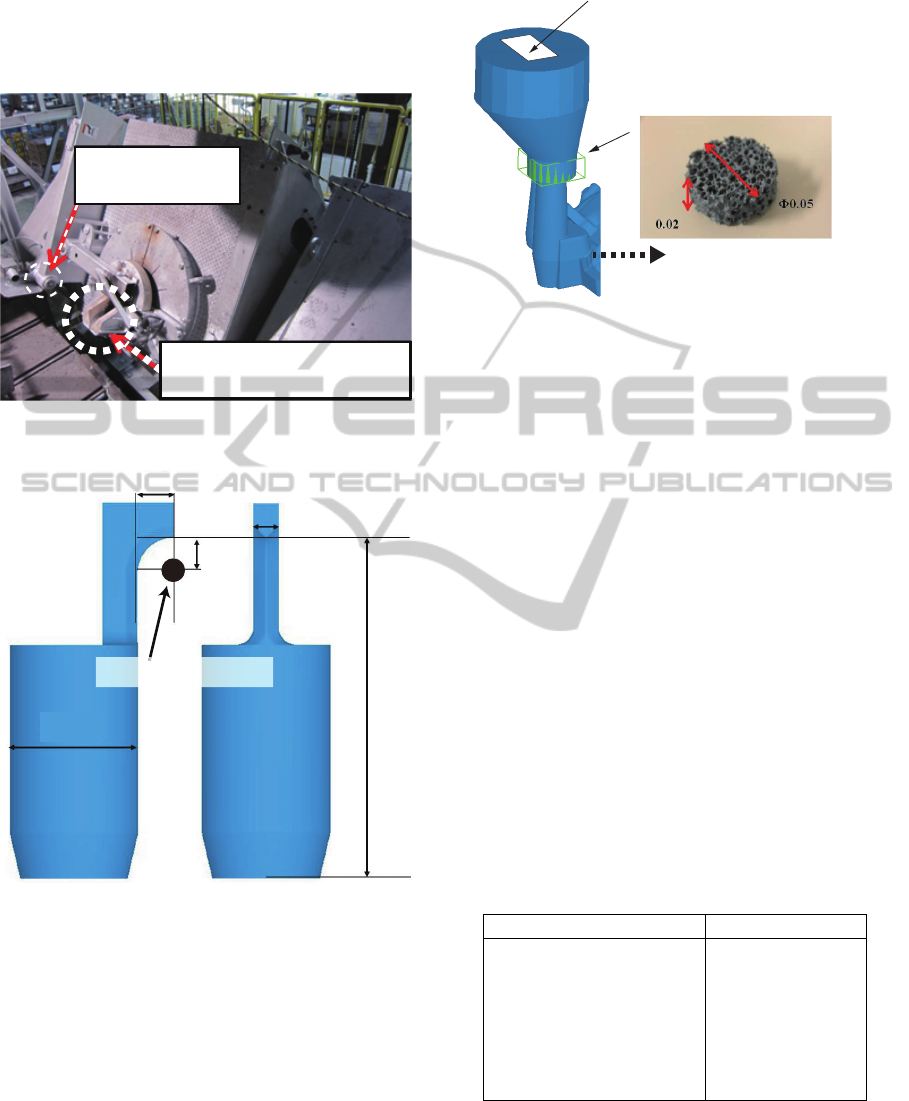
with a melting furnace to control the temperature of
the molten metal. Thus, the viscosity of the molten
metal was maintained. The capacity of the tank was
300[kg].
The central axis
of tilting
The pouring mouth
of ladle
Figure 1: Overview of the automatic pouring machine.
0.1 [m]
0.07 [m]
0.857 [m]
Φ0.36 [m]
0.1 [m]
The center axis of tilting
Figure 2: Measurement of a tank.
Fig.2 shows the measurement of the tank, and
Fig.3 presents an overview of the sprue cup. In Fig.3,
a molten metal filter (wire mesh) is installed in the
sprue runner for the purpose of removing slag.
3 SETTING THE CFD
SIMULATOR
Our fluid analysis software is a 3D fluid calculation
program that uses a calculus of finite differences for
handling a wide range of flows, from the flow of an
Position of the molten metal filter
Flow to the mold
Pouring the molten metel
Figure 3: Overview of a casting mold.
incompressible fluid and flow accompanied by an ad-
justable surface to the flow of a compressible fluid
flow accompanied by solidification. The free sur-
face is calculated using the Volume Of Fluid (VOF)
method(C.W.HirtCB.D.Nichols, 1981). The geom-
etry of complex objects is handled using the Frac-
tional Area Volume Obstacle Representation (FA-
VOR) method(C.W.HirtCJ.M.Sicilian, 1985).
3.1 Setting of the Casting Mold
In this study, cast steel is assumed as the molten
metal, and its fluid properties are shown in Table 1.
The weight of the casted product is 26[kg], and the
volume is 3.65
×
10
−3
[m
3
]. The temperature of the
molten metal in the melting furnace is set to a value
of about 1200
◦
C.
This product has thin-wall parts. Thus, it is ad-
visable to set as fine a mesh as possible. Table 2
shows the minimum settings to perform the calcula-
tions quickly and accurately. This analysis time was
12 hours.
Table 1: Fluid parameters of Ductile Cast Iron.
Fluid parameters Ductile Cast Iron
Density 7620 [kg/m
2
]
Viscosity 0.008 [Pa·s]
Temperature of the Fluid 1873 [K]
Specific Heat 1032 [J/(kg·K)]
Thermal Conductivity 23.2 [W/(m ·K)]
Liquidus Temperature 1769 [K]
Solidus Temperature 1615 [K]
3.2 Setting of the ladle
As seen in Fig.2, the ladle part is symmetrical. Thus,
the analysis area is given as a one-sided model to re-
ICINCO2013-10thInternationalConferenceonInformaticsinControl,AutomationandRobotics
236
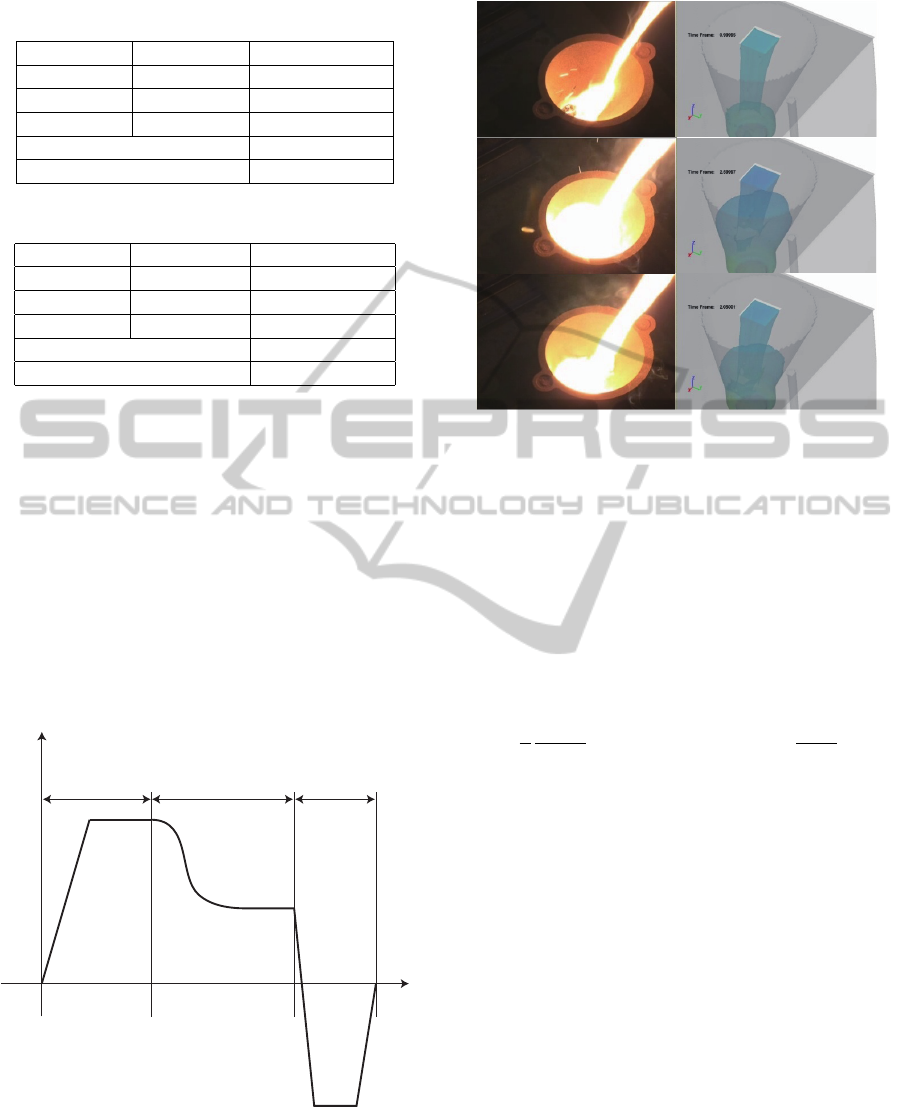
Table 2: Mesh Parameters for sprue cup.
cell size[m] Number of cell
X-direction 0.0016 254
Y-direction 0.0016 153
Z-direction 0.0016 192
Total cell count 7,697,924
Active cell count 772,331
Table 3: Mesh Parameters for ladle.
cell size[m] Number of cell
X-direction 0.01-0.0025 94
Y-direction 0.01 20
Z-direction 0.01-0.025 112
Totalcellcount 240,770
Active cell count 61,104
duce the analysis time. Table 3 shows the minimum
settings to perform the calculations quickly and accu-
rately, and the mesh parameter is set such that a rough
mesh is used around the bottom part of the tank be-
cause the fluid is stable in that section. On the other
hand, a fine mesh is used around the tapping hole be-
cause the fluid velocity is high and the fluid is unstable
in that section.
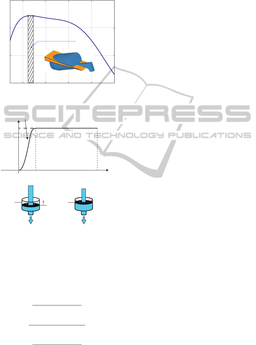
Fig.4 indicates the angular velocity curve of the
ladle. The tilting has three parts. In the first part, the
ladle is tilted until just before outflow. In the second
part, the ladle starts to pour. In the third part, the ladle
is tilted back to stop the pouring.
Stop the poring
Pouring
(Optimization area)
Tilting to start
the pouring
Angular velocity [deg/s]
Time [s]
Figure 4: Tilting motion of the ladle.
3.3 Setting of the Molten Metal Filter
In the CFD simulator, the molten metal filter is set by
using the equation of flow loss as shown in Eq.(1).
Figure 5: Comparison of flow in sprue cup.
To identify the parameter for flow loss, the parameter
of porosity is calculated using Archimedes’ principle.
As a result, the parameter of porosity is V
F
=0.837,
and the diameter of the fiber is d=0.001[m]. The other
parameter is identified by comparing the fluid behav-
ior. As a result, α is 180 and β is 2.0.
Comparing these with the pouring test results as
shown in Fig.5, it can be seen that a satisfactory repro-
duction of the molten metal behavior inside the sprue
was achieved.
K =
µ
ρ
1 −V
F
V
2
F
ADRG(1 −V
F
) + BDRG
ReV
F
d
(1)
ADRG = α/d
2
BDRG = β/d
4 PROPOSED CALCULATION
METHOD
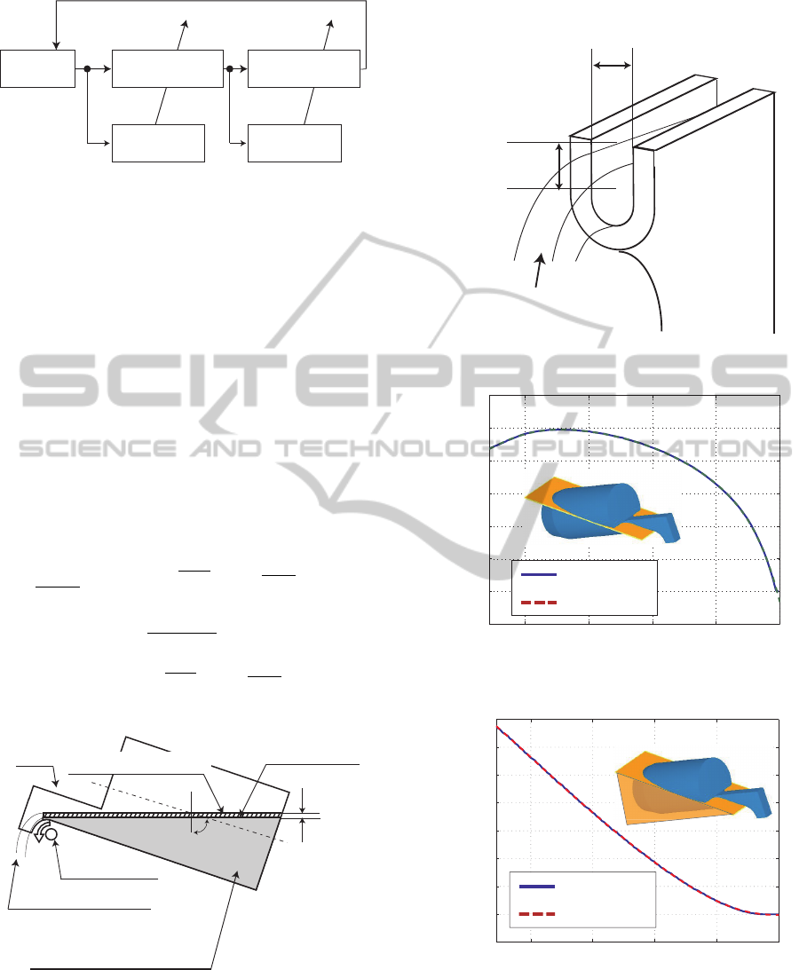
Fig.6 shows the proposed calculation method. In
this method, the mathematic model(Yoshiyuki Noda,
2005)(Yoshiyuki Noda, 2011) and the CFD simulator
are included. The reference angular velocity ω[rad/s]
is derived by optimization method. In this study, ge-
netic algorithm (GA) was applied as a optimization
method. Using this ω[rad/s], the outflow q from the
ladle is calculated by the mathematic model, and the
fluid level h
c
of the cup is calculated by mathematical
model with outflow q. Then, the model errors of the
mathematical model are modified by the CFD simula-
tor. Finally, comparing the maximum fluid level, the
optimization method derives the reference angular ve-
locity, which is a satisfied constraint.
DerivationofControlInputusingOptimizationwithCFDSimulatoranditsApplicationtoaMolten-metalPouringProcess
237
h
c
Mathematical model
of the sprue cup
CFD simulation
of the sprue cup
Mathematical model
of the ladle
CFD simulation
of the ladle
ω
q
f
c
l
c
c
Optimization
method
Figure 6: Proposed claculation method.
4.1 Modeling of the Ladle
Eq.(2) indicates the model of the outflow from the la-
dle. This equation derives the volume of pouring q
f
[m
3
/s] from the angular velocity ω(t) [rad/s] of the la-
dle. Fig.7 and Fig.8 show each variable, where h[m]
is the minimum fluid level from the liquid surface to
the pouring mouth, and V
s
(θ(t))[m
3
] is the residual
volume of fluid. A(θ(t))[m
2
] is the fluid surface, and
L
n
[m] is the width of the pouring mouth. In this equa-
tion, the fluctuation of the fluid affected by fluid be-
havior or the centrifugal force is not considered be-
cause the maximum tilting speed is sufficiently low.
The variables A(θ(t)) and V
s
(θ(t)) are calculated
by fitting curve. Fig.9 and Fig.10 show the analysis
result.
dV
r
(t)
dt
= −c
l
∫
V
r
(t)
A(θ(t))
0
L
f
2gh
b
dh
b
−
∂V
s
(θ(t))
∂θ(t)
ω(t)
q(t) = c
l
∫
V
r
(t)
A(θ(t))
0
L
f
2gh
b
dh
b
(2)
Flow rate q
f
[m/s
2
]
h
b
[m]
V
r
[m]
V
s
[m]
Rotation point
Ladle
Tilting angle θ [deg]
Volume of the outflow
Residual volume of fluid
Surface area A(θ) [m
2
]
Figure 7: Variables for the mathematical model of ladle.
4.2 Modeling of the Sprue
Eq.(3) represents the fluid level model of the sprue
cup. This equation derives the fluid level h
c
from the
Width of Pouring mouth
at height L
f
h
b
[m]
Pouring mouth
of the ladle
Depth from suface
of fluid h
b
[m]
Flow rate q
f
[m/s
2
]
Figure 8: Variables of the pouring mouth.
70 75 80 85 90
-0.05
0
0.05
0.1
0.15
0.2
0.25
0.3
Angle [deg]
Surface area A [m
2
]
Fitted curve
CFD analysis
Figure 9: Surface area A at the angle θ.
70 75 80 85 90
-0.005
0
0.005
0.01
0.015
0.02
0.025
0.03
0.035
Angle [deg]
Residual volume of fluid V
s
[m
3
]
Fitted curve
CFD analysis
Figure 10: Volume of fluid V
s
at the angle θ.
volume of pouring q
f
. Fig.11 shows each variable,
where h
c
is the fluid level at the timet, A
c
is the fluid
surface, A
Exit
is the area of bottom of the cup, q
Exit
is the outflow to the mold, and h
re f
is the maximum
ICINCO2013-10thInternationalConferenceonInformaticsinControl,AutomationandRobotics
238
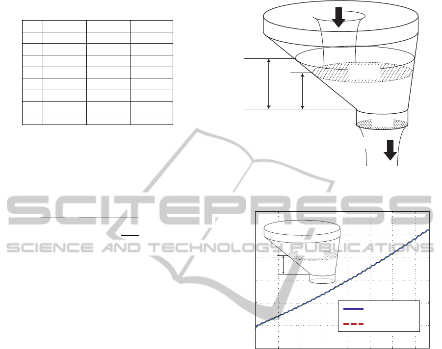
Table 4: Parameters of the fitting curve.
A V
s
A
c
a
1
0 3.2e
−
11 0
a
2
0 0 0
a
3
-3.0e
−
4 0 0
a
4
-3.8e
−
2 -7.0e
−
4 -1.0e
−
4
a
5
-2.9 5.6e
−
2 4.0e
−
4
a
6
134.4 -2.8 6.0e
−
4
a
7
-3431.9 77.4 1.4e
−
3
a
8
37506.3 -912.3 3.8e
−
3
liquid level.
The variables A
c
is calculated by fitting curve. The
analysis result are shown in Fig.12.
The fitting curve is shown in the Eq.4, and the pa-
rameters are shown in Table 4.
dh
c
(t)
dt
=
q
f
(t) − q
Exit
(t)
A
(h
c
)
q
Exit
(t) = c
c
∗ A
Exit
2gh
c
(3)
y = a
1
x
7
+ a
2
x
6
+ a
3
x
5
+ a
4
x
4
+ a
5
x
3
+a
6
x
2
+ a
7
x
1
+ a
8
(4)
5 OPTIMIZATION OF THE
ANGULAR VELOCITY CURVE
5.1 Derivation the pouring Start Angle
and End Angle
The pouring angle area is determined by the pouring
start angle θ
a
and end angle θ
b
, by which the molten
metal can be poured to fill the reference volume with
least displacement angle. Eq.(5) represents the for-
mula for the computation, and Fig.13 shows the vol-
ume change of fluid per degree. In this figure, ρ is
density and M is the mass of the produced unit. In
this study, M is 24.1[kg]. As the analysis result, start
angle θ
a
is 71.1[deg], and end angle θ
b
is 72.3[deg].
θ
min
= min
θ
b
− θ
a
;M ≈ ρ
∫
θ
b
θ
a
A(θ)dθ
(5)
5.2 Equation of Reference Fluid Level
Curve
In this study, the fluctuation of fluid level are derived
in two parts as shown in Fig.14. The first part is for
h
c
(t)
h
ref
(t)
A
Exit
A
c
(h
c
)
q
f
(t)
q
Exit
(t)
Figure 11: Variables for the mathematical model of the
sprue cup.
0 1 2 3 4 5 6 7
2
4
6
8
10
12
14
x 10
-3
Fluid level h
c
[m]
Surface area at the fluid level A
c
[m
2
]
h
c
(t)
A
c
(h
c
)
Fitted curve
CFD analysis
Figure 12: Surface area at the fluid level h
c
.
the rising of the liquid, the second part is for the equi-
librium of the liquid, where t
end
is the finish time of
the rising of the liquid, T
s
is the finish time of pouring,
h
m
is the reference height.
The reference fluid level velocity curve of the ris-
ing part is defined by Eq.(6)∼Eq.(8), where t is the
time and, a
i
(i = 0 ∼ 7) are the constants.
f (t) =
n
∑
i=0
a
i
t
i
(6)
f
′
(t) =
n−1
∑
i=0
(a
i+1
t
i
)(i + 1) (7)
f
′′
(t) =
n−2
∑
i=0
(a
i+2
t
i
)(i
2
+ 3i + 2) (8)
The initial conditions are f (0)=0.0[m],
f
′
(0)=0.0[m/s], f
′′
(0)=0.0[m/s
2
], the conditions
at t=t
end
are f (t
end
)=h
m
[m], f
′
(t
end
)=0.0[m/s],
f
′′
(t
end
)=0.0[m/s
2
]
DerivationofControlInputusingOptimizationwithCFDSimulatoranditsApplicationtoaMolten-metalPouringProcess
239
0
1
2
x 10
-4
Angle [deg]
Volume change of fluid per degree [m
3
/deg]
70 75 80 85 90
ρ V = 24.1 [kg]
θ
a
θ
b
Figure 13: Volume change of fluid per degree.
Fluid height [m]
Rising part
Rising part
Equilibrium part
Equilibrium part
Time [s]
h
m
h
c
h
m
t
end
T
s
h
m
Figure 14: Reference fluid level curve.
Therefore, (9) is solved by substituting the initial
conditions into (6) ∼ (8).
a
0
= a
1
= a
2
= 0 (9)
From the conditions at t=t
end
, (10)∼(12) are also
given as
a
5
=
6h
m
− 6a
7
t
1
7
− 3a
6
t
1
6
t
1
5
(10)
a
4
=
−15h
m
+ 8a
7
t
1
7
+ 3a
6
t
1
6
t
1
4
(11)
a
3
=
10h
m
− 3a
7
t
1
7
− a
6
t
1
6
t
1
3
(12)
where the t
end
,h
m
,a
7
,a
6
are unknown parameters
solved by optimization problem using GA.
5.3 Formulation of Design
Specifications
The specification of the reference fluid level curve are
formulated by making use of penalty functions, and
then t
end
,h
m
,a
7
,a
6
are simultaneously calculated to
satisfy the specifications. In this design, Specs.(I)-
(III) shown below were given.
Spec.(I): The maximum angular velocity of the
ladle do not exceed the pouring machine constraint.
Penalties are given if the following relation is not sat-
isfied.
max(ω
t
) > 0.14 [rad/s] (13)
Spec.(II): The allowed pouring time T
s
do not ex-
ceed the production constraint. Penalties are given if
the following relation is not satisfied.
T
s
> 5 [s] (14)
Spec.(III): The spilling liquid Q
spill
[m
3
] from the
sprue cup is more than 0 [m
3
], where this spec is eval-
uated by using CFD simulator. Penalties are given if
the following relation is not satisfied.
Q
spill
> 0 [m
3
] (15)
The unknown parameters of t
end
,h
m
,a
7
,a
6
are ob-
tained by minimizing the cost function expressed as
J
s
= T
s
+ J
p
(16)
In (16). T
s
is the settling time of the transfer ex-
pressed as follows Eq.(17), and J
p
is the penalty term
expressed as Eq.(18)
T
s
=
{
t| ρ · q
Exit
(t) = M
}
(17)
J
p
= J
I
+ J
II
+ J
III
(18)
where J
i
= 10
8
(i =Spec.(I), Spec.(II), Spec.(III) )
is the penalty. Each time the penalty conditions hold,
the penalty, which is big enough to avoid the penalty
conditions, will be added to satisfy the specifications.
In order to obtain the reference fluid level curve, the
optimization problem with the constraints is formu-
lated with: the target function (the poring time T
s
−→
minimum) and the constraints Eq.(13) ∼ Eq.(15). In
the Eq.(10)∼ Eq.(12), t
end
,h
m
,a
7
,a
6
are unknown pa-
rameters. The unknown parameters are computed by
solving the optimization method with the constraints
expressed in Eq.(16).
To optimize the cost function, the GA is applied to
the present problem because there are four unknown
parameters in this case. Table 5 shows the genetic
algorithm parameters.
ICINCO2013-10thInternationalConferenceonInformaticsinControl,AutomationandRobotics
240
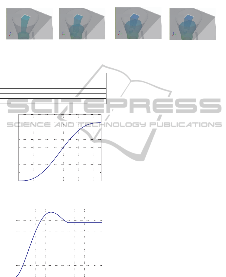
0.2s
0.8s
0.6s
0.4s
Simulation
Figure 17: Fluid behavior of the fluid in the sprue cup by using CFD simulation.
Table 5: Parameters for genetic algorithms.
Number of population 30
Number of elite preservation 2
Crossover fraction 80[%]
Mutation evolution 5[%]
Crossover One-point crossover
Selection Roulette wheel selection
0 0.1 0.2 0.3 0.4 0.5
0
0.02
0.04
0.06
0.08
0.1
0.12
0.14
0.16
Time[s]
Fluid level [m]
Figure 15: Optimum reference fluid level curve.
0
0.1 0.2 0.3 0.4 0.5 0.6 0.7 0.8
0
1
2
3
4
5
6
x 10
-3
Time[s]
Outflow from the ladle q
f
[m
3
/s]
Figure 16: Outflow from the ladle.
6 OPTIMIZATION RESULT
The calculation time was 32 hours until the finish.
the number of iterations of the convergence is around
33, and the settling time is converged at 1.49[s].
As a result of the computations, each parameter is
t
end
=0.546[s], h
m
=0.136[m], a
7
=0.258, a
6
=0.810 ,
a
5
=14.925, a
4
=-21.772, a
3
=8.1169. The intended ref-
erence fluid level curve is shown in the Fig.15, and
Fig.16 shows a simulation result of outflow from the
ladle using the reference fluid level curve. Comparing
the calculation time to the iterative learning control,
the latter required 5 [days] to obtain the same result.
Thus, it can be said that the calculation speed was im-
proved. Fig.17 shows a result of the CFD simulation.
In this figure, the liquid level can be controlled at a
fixed high level.
7 CONCLUSIONS
The aim of this study was to design a calculation
method using the CFD simulator with optimization
method. This proposed method was applied to an ac-
tual problem of a tilting-type automatic pouring ma-
chine, and derived the pouring speed by which a sprue
cup could be swiftly filled and the liquid level con-
trolled at a fixed high level. The proposed method
could derive the expected flow rate, and the calcula-
tion time was 32 hours from start to finish. The iter-
ative learning control required 5 [days] of calculation
to obtain the same result. Thus, it can be said that the
calculation speed was improved.
REFERENCES
C.W.HirtCB.D.Nichols (1981). Vokume of fluid (vof)
method for the dynamics of free boundaries. In Jour-
nal of Computational Physics. Elsevier.
C.W.HirtCJ.M.Sicilian (1985). A porosity technique for the
definition of ovstacles in rectangular cell meshues. In
DerivationofControlInputusingOptimizationwithCFDSimulatoranditsApplicationtoaMolten-metalPouringProcess
241

Proc. of 4 th International Conference on Ship Hydro-
dynamics. Naval Architecture and Marine Engineer-
ing.
Martin, P. S. P. C. M. (2005). Integrating multibody sim-
ulation and cfd : toward complex multidisciplinary
design optimization. In JSME international journal.
Japan Society of Mechanical Engineers.
T.Sakuragi (2004). Prediction of gas defects by mold-filling
simulation with consideration of surface tension. In
J.JFS. Japan Foundry Engineering Society.
Y. Kuriyama, K. Y. and Watanabe, M. (2009). Solution
search algorithm for a cfd optimization problem with
multimodal solution space. In Proc. of World Foundry
Congress. WFC.
Y.Kurokawa, N. and H.Ota (2001). Classification of pin
hole defect of iron casting. In J.JFS. Japan Foundry
Engineering Society.
Yoshiyuki Noda, Kenfichi Yano, K. T. (2005). Control of
self-transfer-type automatic pouring robot with cylin-
drical ladle. In 16th IFAC World Congress. IFAC.
Yoshiyuki Noda, Michael Zeitz, O. S. K. T. (2011). Flow
rate control based on differential flatness in automatic
pouring robot. In CCA 2011. IEEE.
ICINCO2013-10thInternationalConferenceonInformaticsinControl,AutomationandRobotics
242
