Magnitude Sensitive Image Compression

Enrique Pelayo, David Buldain and Carlos Orrite

Aragon Institute of Engineering Research, Zaragoza University, Mariano Esquilor, Zaragoza, Spain

Keywords:

Image Compression, Competitive Learning, Neural Networks, Saliency, Self Organizing Maps, JPEG, DCT.

Abstract:

This paper introduces the Magnitude Sensitive Competitive Learning (MSCL) algorithm as a reliable and efﬁ-

cient approach for selective image compression. MSCL is a neural network that has the property of distributing

the unit centroids in certain data-distribution zones according to a target magnitude locally calculated for every

unit. This feature can be used for image compression to deﬁne the block images that will be compressed by

Vector Quantization in a later step. As a result, areas of interest receive a lower compression than other parts

in the image. Following this approach higher quality in the salient areas of a compressed image is achieved in

relation to other methods.

1 INTRODUCTION

In the human vision system the attention is attracted to

visually salient stimuli and therefore only scene loca-

tions sufﬁciently different from their surroundings are

processed in detail. This provides the necessary mo-

tivation to devise a novel image compression method

capable of applying distinct compression ratios to dif-

ferent zones of the image according to their saliency.

In this paper we make use of the Magnitude

Sensitive Competitive Learning Algorithm (MSCL)

(Pelayo et al., 2013). MSCL is a Vector Quantization

method based on competitive learning, where units

compete not only by distance but also by a user de-

ﬁned magnitude. Using saliency as the magnitude,

units tends to model more accurately the salient ar-

eas of the images, and therefore the neural network

behavior imitates the human vision system.

Vector quantization (VQ) is a classical quantiza-

tion method. In the context of image processing, basic

vector quantization consists in dividing the input im-

age into blocks of pixels of a pre-deﬁned size, where

each block is considered as a d-dimensional vector.

Each of these input vectors from the original im-

age is replaced by the index of its nearest codeword.

Only this index is transmitted through the media. The

whole codebook serve as a database known on the re-

construction site. This scheme reduces the transmis-

sion rate while maintaining a good visual quality.

In VQ, compression level depends on two factors,

the number of blocks and the level of compression of

each block. Both factors are related in an inverse way.

As less number of blocks are higher is the bit depth

necessary to codify each block for a similar quality.

Some authors (Laha et al., 2004), (Amerijckx

et al., 2003), (Harandi and Gharavi-Alkhansari, 2003)

and (Liou, 2007) have already used some VQ vari-

ants, such as Kohonen neural network (Kohonen,

1998) for image compression. These algorithms use a

ﬁxed block size and concentrate in several ways to get

a smaller codiﬁcation of each block or to improve the

quality of the codiﬁcation. Laha (Laha et al., 2004)

uses surface ﬁtting of data assigned to each codeword

instead of the codeword itself, which improves the vi-

sual quality of the results. (Amerijckx et al., 2003),

(Harandi and Gharavi-Alkhansari, 2003) and (Liou,

2007) apply DCT ﬁltering (Ahmed et al., 1974) to

each block previous to the quantization step to lower

the dimension of the input data. On the other hand,

(Amerijckx et al., 2003) takes advantage of the topo-

logical ordering property of the SOM neural network

to codify indexes with a few bytes.

In this paper blocks may have different size, cho-

sen according to its relevance (which is selected fol-

lowing the image saliency). Blocks located in areas of

high image saliency are smaller than those assigned

with low saliency. As bit depth used in the quantiza-

tion step is the same for all blocks, quantization error

increases directly with the block size in areas of low

image saliency. Therefore, a lower number of blocks

are used to represent the whole image increasing the

overall image compression and preserving at the same

time the quality of most relevant areas.

One important difference from these methods is

370

Pelayo E., Buldain D. and Orrite C..

Magnitude Sensitive Image Compression.

DOI: 10.5220/0004552103700380

In Proceedings of the 5th International Joint Conference on Computational Intelligence (NCTA-2013), pages 370-380

ISBN: 978-989-8565-77-8

 2013 SCITEPRESS (Science and Technology Publications, Lda.)

that, in our approach, block shape is, in general, ir-

regular, i.e., neither rectangular nor squared.

The remainder of this paper is organized as fol-

lows. Section 2 describes the MSCL algorithm. Sec-

tion 3 shows its use to achieve selective image com-

pression focused on the most salient regions of an im-

age with the method that we call Magnitude Sensitive

Image Compression (MSIC). A comparative between

MSCL and classical JPEG and SOM based VQ algo-

rithms for a high compression ratio task is carried out

in Section 4. Finally, Section 5 concludes with a dis-

cussion and ideas for future work.

2 THE MSCL ALGORITHM

MSCL is a type of artiﬁcial neural network that is

trained using unsupervised learning to produce a rep-

resentation of the input space of the training sam-

ples depending on a magnitude. Prototype of unit

i (i = 1 . .. M) is described by a vector of weights

(t) = (w

, .., w

) in a d-dimensional space, and the

magnitude value MF(i, t). This function is a mea-

sure of any feature or property of the data inside the

Voronoi region of unit i, or a function of the unit pa-

rameters.

The idea behind the use of this magnitude term is

that, in the units, the winner will be the unit with the

lowest magnitude value. As a result of the training

process units will be forced to move from the data re-

gions with low MF(i,t) values to regions where this

magnitude function is higher. MSCL follows next

steps:

2.1 Global Unit Competition

Two units { j

, j

} with minimum distance from their

weights to the input data vector x(t) are selected as

winners in this step:

∥x(t) − w

(t)∥ < ∥x(t) − w

(t)∥,

∀i ̸= k ∧ k ∈ { j

, j

} (1)

2.2 Local Unit Competition

In the second step, ﬁnal winner unit j is selected from

units belonging to { j

, j

} as the one that minimizes

the product of its Magnitude Function and the dis-

tance of its weights to input data vector:

j = argmin(MF(k, t) · ∥x(t) − w

(t)∥),

k ∈ { j

, j

} (2)

2.3 Winner Updating

Only winner’s weights are adjusted as follows:

(t + 1) = w

(t) + α(t)(x(t) − w

(t)) (3)

where α(t) is the learning factor forced to decay with

iteration time t. After that the new magnitude function

MF( j, t) is calculated for this new codeword value.

Winner j is called the best matching unit (BMU).

3 MAGNITUDE SENSITIVE

IMAGE COMPRESION

Figure 1 shows the whole MSIC algorithm applied to

grayscale images, where image compression, in the

transmitter, is represented on the top and the image

restoration process at the receiver is depicted on the

bottom. Image is compressed with different quality

according to a selected user magnitude. Subsection

3.6 explain how to extent this methodology to color

images.

In this work we use as magnitude the saliency

map, with the same size as the processed image, pro-

vided by a user function. Section 4 explain the func-

tions used in this work.

The results of the compression are a group of im-

age blocks encoded by indexes. Unlike other image

compression methods, our algorithm uses blocks of

different sizes, which are located in any position of

the image. Therefore, this implies that block centers

and sizes has to be sent to the receiver, apart from the

corresponding index. As this approach would mean

the transmission of huge quantity of information, we

have adopted an alternative solution.

We use the saliency map to train a MSCL network,

using as inputs the coordinates (x

, x

) of each pixel

and the saliency as magnitude. After training, the

weights of its units (codewords) are the block cen-

ters (bc(k), k = 1 ..N

).. The surrounding assigned to

the Voronoi region of each block-center conﬁgure the

corresponding blocks. The image is so fragmented in

so many blocks as units in this network (N

). In sub-

section 3.1 we will show how to determine the block

sizes (and block limits) for each codeword or unit.

This process encodes the saliency map with low qual-

ity, and both the encoded image and the encoded map

are transmitted.

At the receiver ﬁrst the saliency map is regener-

ated, and with it, the image block limits and centers

can be calculated. They are used with the image in-

dexes to restore the image.

MagnitudeSensitiveImageCompression

371

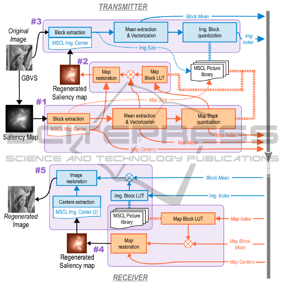
Figure 1: Global algorithm for grayscale images. Marked with #n the corresponding subsection with the detailed explanation

and, also showing the order of processing steps in the transmitter and receiver.

It is worth noting that it is necessary an additional

step at the transmitter. Instead of using directly the

saliency map to extract the image blocks, we ﬁrst de-

code a saliency map from the encoded map that has

to be transmitted. Then we calculate the image cen-

ters and limits of image blocks using this Regenerated

Saliency Map that will be also regenerated by the re-

ceiver.

Summarizing the MSIC algorithm steps are:

1. Map quantization (at transmitter).

2. Map restoration (at transmitter).

3. Image quantization (at transmitter).

4. Map restoration (at receiver).

5. Image restoration (at receiver).

MSIC algorithm uses several MSCL networks:

MSCL

(map center) to extract map blocks,

MSCL

(image center) to extract image blocks, and

a pool of MSCLs that he call MSCL picture li-

brary (MSCL

PIC

) to generate indexes that encode each

block pixels, and act as Look-Up-Table to decode the

block shapes with these indexes. The ﬁrst and second

neural networks are trained online during map and im-

IJCCI2013-InternationalJointConferenceonComputationalIntelligence

372

age quantization. Their codewords are the block cen-

ters. However MSCL

PICT

form a codebook database

that is trained ofﬂine. It is known by the transmitter

and the receiver as a library of the method. Finally re-

ceiver uses another MSCL (MSCL

IC2

), that becomes

identical to MSCL

when trained at receiver.

Following sections explain the process in detail.

3.1 Saliency Map Quantization

The idea is to consider the saliency map as an image

and apply the same compression steps that will be ap-

plied to the image.

First step corresponds to the block extraction from

the saliency map according to the saliency values.

We train a MSCL network (MSCL

) using as inputs

the 2D coordinates of each pixel(x) and as magnitude

function:

MF(i,t) =

∑

saliency(x

)

(t)

(4)

where x

are the data samples belonging to the

Voronoi region of unit i at time t, V

(t) is the num-

ber of samples in the Voronoi region, and saliency(x)

is the pixel saliency of the corresponding sample.

Trained unit weights correspond to the coordinates of

the unit in the image, and the magnitude value is the

mean of the saliency inside its Voronoi region. Once

trained, it is possible to ﬁnd the best matching unit

(BMU

) assigned to every pixel (using magnitude

during competition). The block assigned to each unit

is the rectangle wrapping its Voronoi region. A block

mask of equal size than the block is also provided

in order to mark the pixels belonging to that irregu-

lar Voronoi region, see Fig. 2. We used 40 units for

MSCL

in our experiment. With this small number

of units a coarse saliency map is obtained, but it is

enough to deﬁne areas with high saliency.

To codify each of the blocks by VQ, we ﬁrst re-

size the block to a squared shape with side value

as the maximum between its horizontal and vertical

block sizes. The block and the mask are inserted in

the squared image ﬁlling with zeros the void rows or

columns. After that, both are resized to a vector form.

We use mean-removed vectors to have a better quan-

tiﬁcation. Mean value of saliency in each block of

pixels, that we call mean block-saliency (m

(x, y)), is

sent encoded by 7 bits.

The resulting vector is separated according to its

size and dispatched for training or testing to the

MSCL picture library (MSCL

PICT

(l)). This pool of

codebooks are trained separately only once and be-

come a lookup table in the algorithm. In order to

avoid the transmission of the whole codebook pool

it is known by both the transmitter and the receiver.

Each codebook of the pool, with 256 codewords,

is dedicated to a precise input-vector length. This

election of the same number of codewords for differ-

ent block sizes forces that larger blocks present less

detail in pictorial content than smaller blocks. We

have chosen a limited group of sizes that model sev-

eral size possibilities (the value of l is the length of

the square edge to which we have resized the block):

l = [4, 6, 7, 8, 10, 15, 29] (5)

This pool of codebooks can be specialized in the

type of images considered in the transmission task, or

can be generated using an universal library of training

images. The images for training are processed follow-

ing previous described steps, but the magnitude func-

tion chosen for these MSCL

PICT

(l) networks is the hit

frequency of each unit, that is:

MF(i,t) = hits(i, t) (6)

During competition the BMU

PICT

is calculated

taking into account the mask vector in order to avoid

the zero-padding mentioned before. Each time a

sample is presented to each neural network of the

pool, the corresponding mask is also presented, and

only masked weight components are used to compete

(see Fig.2, Right). Each sample might have different

masked components. In this way, only pixels corre-

sponding to the Voronoi region of a block are used to

ﬁnd its BMU

PICT

At the end of this step, the magnitude map has

been divided in 40 blocks. We have to send to the re-

ceiver the following information of each block: Map

indexes (BMU

PICT

) (1 byte), Map mean (7 bits) and

Map Centers (2 bytes). Size of each block is not nec-

essary because it is calculated with the block centers

and magnitude.

3.2 Map Restoration at Transmitter

Map representing the saliency of the image is also re-

stored at transmitter with the information generated

at the previous step. This is because the restored map

will be used at both transmitter and receiver to de-

ﬁne the block centers of the image, so results are the

same in both sides. Map restoration is accomplished

following the previous step in inverse order. First

we calculate Voronoi regions assigned to each of the

Map Centers by searching the BMU

of each pixel

in MSCL

. The codewords of this neural network

are the Map Centers. Additionally, we calculate block

limits and mask wrapping by a rectangle the area cor-

responding to the Voronoi region of each center.

MagnitudeSensitiveImageCompression

373

Figure 2: Neural networks used in the MSIC algorithm: Top: BMU

and BMU

. It is important to mention that this last

MSCL is used also in receiver (BMU

IC2

). Bottom: Block extraction phase. Each block delivers the block limits, the image and

a binary mask. MSCL

PICT

(l) neural network, where a input sample (vectorized block from the extraction phase) has several

masked components.

With the i index of the new block, it is converted

again into an image block by the look-up table created

with MSCL

PICT

(l). The codeword of the BMU

PICT

consists of the pictorical content of the block im-

age, but needs to be displaced with the mean block-

saliency value of the corresponding block. After sum-

ming the mean, it is masked by the binary mask and

added to the regenerated saliency map. Repeating the

process for all the blocks we obtain the regenerated

saliency map, that will represent the saliency values

of pixels for the reconstructed image.

3.3 Image Quantization

A similar strategy to the previous described step is fol-

lowed for image quantization. Blocks are extracted

training the MSCL

(with the coordinates at each

pixel) to get the image block centers according to the

Regenerated Saliency Map at the transmitter. Then

the Voronoi regions of each of these centers are calcu-

lated. Blocks are extracted and vectorized. After re-

moving the mean, each image block is processed with

the MSCL

PICT

(l) that corresponds its size, in order

to use the most similar pictorial content of the library

that will be included in the reconstructed image. It is

only necessary to send for each block, the correspond-

ing block mean and index from the MSCL

PICT

(l).

3.4 Map Restoration at Receiver

Map restoration at receiver is accomplished follow-

ing exactly the same process than map restoration at

transmitter. To do it, the receiver uses for each block

its Map index, mean block-saliency, block-center and

the same ofﬂine MSCL

PICT

(l) picture library. As op-

erations are the same and they are applied to the same

data, the Regenerated Saliency Map at receiver is ex-

actly the same than the one at the transmitter.

3.5 Image Restoration

Last step in the whole process is image restoration,

using the received means of block-saliency, the pixel

indexes and the regenerated saliency map. This step

is similar to the previous described Map restoration

with small changes.

The main difference is that the image block cen-

ters are not available (they have not been transmitted).

They are calculated training a new MSCL (MSCL

IC2

with the coordinates of each pixel, and the magnitude

values in the Regenerated Saliency Map (magnitude

that was calculated with equation 4 at the emitter).

This neural network becomes identical to MSCL

The weights of MSCL

IC2

are the centers of the image

blocks, and their Voronoi regions deﬁne the masks

IJCCI2013-InternationalJointConferenceonComputationalIntelligence

374

and limits.

Once again, image indexes are presented to the

look-up table created with MSCL

PICT

(l) (according

to the block size) that returns the block shape. Fi-

nal image is regenerated by adding means of block-

saliency, masking each block and positioning it in the

image (adding it to the regenerated image as we had

done before with the saliency map).

3.6 Extension to Color Images

Figure 3 deﬁnes the ﬂowchart to use MSCL in the

case of color images. The process is similar to the

used in the case of grayscale images, but applied to

each of the color components of the image.

First, we calculate the saliency map from the color

image. With this saliency map we extract and quan-

tify blocks as described in subsection 3.1, blocks

which were restored at transmitter as mentioned in

3.2. As a result of this step we get the map block-

centers, block-means and indexes. Encoding is made

with the previously trained MSCL

PICT

(l) picture li-

brary.

Then, original RGB image is transformed to the

L-a-b color space. The reason of selecting this color

codiﬁcation is that it has been demonstrated its suit-

ability for interpreting the real world (Cheung, 2005).

Now with these L-a-b color components of the im-

age, we follow the process indicated in 3.3. Each

of them will be trained with a MSCL neural net-

work (MSCL

IC−L

, MSCL

IC−a

, MSCL

IC−b

,) and it will

return the block sizes and indexes for each compo-

nent. The indexes of the blocks are also encoded with

MSCL

PICT

(l).

Once at receiver saliency map is restored (see

3.4). Then, we follow the image restoration

step, applied to each L-a-b component. Its cen-

ters are calculated training three MSCL networks

(MSCL

IC2−L

, MSCL

IC2−a

, MSCL

IC2−b

,), with the co-

ordinates of each pixel, and the regenerated saliency

map. These neural networks becomes identical to

those at the transmitter.

To get the ﬁnal image, we transform the restored

L-a-b image to RGB.

4 EXPERIMENTAL RESULTS

4.1 Grayscale Images

Simulations were conducted on four 256x256 gray

scaled images (65536 bytes), all of them are typical

in image compression benchmarking tasks.

We applied the MSIC algorithm, with the follow-

ing MSCL training parameters: 15 cycles and learn-

ing factor varying along the training process from

0.9 to 0.05. We used Graph-Based Visual Saliency

GBV S(x) ( (Harel et al., 2006) ) as the pixel saliency

of the corresponding sample. However, it is possible

to use other kind of magnitudes to deﬁne which areas

of the image are compressed more or less deeply.

JPEG was done with the standard Matlab imple-

mentation and a compression Quality of Q = 3 or Q=5

(i.e., with a high compression ratio).

We also compare with the algorithm described in

(Liou, 2007), whose main steps are followed for all

the mentioned SOM based algorithms: The original

image is divided into small blocks (we select a size

of 8x8 to achieve a similar compression ratio to JPEG

or MSCL). The 2-D DCT is ﬁrst performed on each

block. The DC term is directly send for reconstruc-

tion. The AC terms after low-pass ﬁltering (we only

consider 8 AC coefﬁcients) is fed to a SOM network

for training or testing. All experiments were carried

out with the following parameters: 256 units, 5 train-

ing cycles and learning factor decreasing from 0.9 to

0.05.

The number of bytes used to compress each image

was the same for MSCL and JPEG (see table 1) and

ﬁxed to 2048 for SOM.

For evaluation purpose, we use the mean squared

error (MSE) as an objective measurement for the per-

formance. Table 1 shows the resulting mean of the

MSE in 10 tests using our algorithm compared to

JPEG and SOM applied to 4 test images. We present

a second column showing the value of MSE but only

calculated in those pixels which saliency is over 50%.

Standard deviation is also shown (in brackets).

To obtain the generic pictorial library

MSCL

PICT

(l) we used three additional images

from the (Computer Vision Group, 2002) with the

same training parameters. This number is quite low,

but enough to show the good performance of our

proposal. However, in a real scenario it would be

necessary to use a higher number of images to get a

suitable pictorial library. Moreover, we have not used

any entropic coding applied to indexes which would

have result in a further compression.

As expected, the MSE value calculated for the

whole image area given by JPEG is lower than the one

provided by MSIC, because prototypes tend to focus

on zones with high saliency while other areas in the

image are under-represented.

However, when MSE was calculated taking into

account only those pixels with high saliency, MSIC

obtained better results than JPEG or SOM. This ef-

fect can be clearly appreciated by visual inspection of

MagnitudeSensitiveImageCompression

375

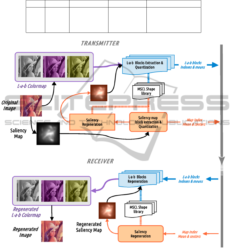
Table 1: Mean MSE for the whole image as well as for areas with saliency over 50% (grayscale example).

Image Q/Bytes JPEG(Tot/50%) SOM(Tot/50%) MSIC(Tot/50%)

Lena Q5/2010 212.3/340.4 205.4/374.0 501.1(18.2)/211.0(6.1)

Street Q5/2127 302.3/369.0 322.1/465.3 466.2(7.8)/210.6(4.2)

Boat Q5/1988 263.9/383.7 280.4/486.6 436.4(12.3)/282.0(5.6)

Fish Q3/2090 485.7/597.7 466.3/904.3 895.8(15.8)/254.2(9.6)

Figure 3: Global algorithm for color images. Each color component is processed separately as in the grayscale method.

However this process is exempliﬁed with a different magnitude deﬁnition for the saliency map, oriented to preserve the detail

of the image for certain colors selected by the user.

the images represented in Figure 4. They show how

MSIC achieves a higher detail level at image areas of

high saliency. In the case of JPEG, it tends to ﬁll up

big portions of the image with plain blocks, being un-

able to obtain a good detail at any part of the image.

On the other hand, SOM produces slightly blurred im-

ages due to the low frequency ﬁltering.

The new algorithm could also be used in com-

pression applications with other magnitude functions

instead of saliency. Figure 5 shows the compressed

results of applying MSIC using different Magnitude

Functions to the street image. From left to right, ﬁrst

image is the original one, second image is MSIC us-

ing the same Magnitude Functions than the one used

IJCCI2013-InternationalJointConferenceonComputationalIntelligence

376

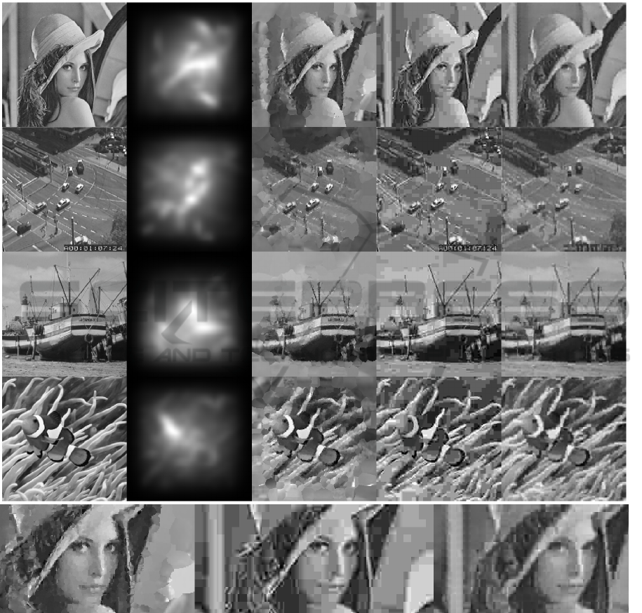
Figure 4: Top in columns: Original image, saliency map, MSIC, JPEG and SOM compression for the test images. Bottom:

Lena detail in the three methods. It can be clearly seen that the Lena face, compressed with MSIC shows a more natural view

(altmost like painted with Pointillism technique) than the other methods that have square block borders.

in equation 4. The Magnitude function in third image

is the same of equation 4, but using 1 − GBV S(x) in-

stead of the pixel saliency of the corresponding sam-

ple. The fourth image uses the value of the vertical

coordinate (normalized to one) and ﬁnally the ﬁfth

one uses the value of the vertical coordinate (normal-

ized to one) minus one. It can be clearly seen that

depending on the deﬁned Magnitude Function, cer-

tain areas are compressed in with quality (foreground,

background, top or bottom of the image).

This toy example was only presented to show

the possibilities of achieving selective compression in

different areas of the image just by varying the Mag-

nitude Function.

4.2 Color Images

In the color experiments, it is applied the same

method explained in section 3.6, with the same pa-

rameters used in the grayscale case.

We use a different saliency deﬁnition focused

in those image zones with colors selected by the

user.This type of compression, preserving with more

detail image zones with certain color selection, may

MagnitudeSensitiveImageCompression

377

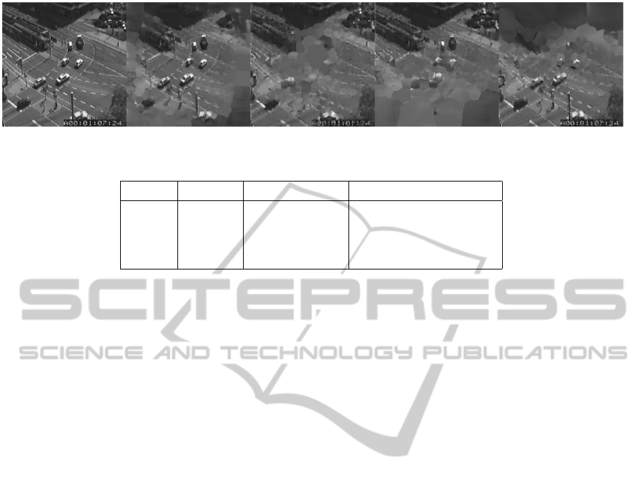
Figure 5: Original ’Street’ image and the compressed images using MSIC with four different Magnitude Functions.

Table 2: Mean MSE for the whole image as well as for areas with saliency over 50% (color example).

Image Q/Bytes JPEG(Tot/50%) MSIC(Tot/50%)

Fish Q3/1702 1328/2695 2193(20.7)/1789(40.3)

Flower Q5/1722 862/1299 3540(227.1) /1167(49.4)

Boat Q6/1720 1303/1570 2366(87.4)/1190(25.3)

Sky Q5/1706 967/2312 240(58.2) /468(19.7)

have different applications. For instance, in medical

images, the specialist may deﬁne the colors of those

areas that has to be well preserved. Other applica-

tion is in video transmission limited by narrow band-

widths, as in underwater image transmission. In that

case it is possible to work with a high compressed

global image, and if the user wants a higher deﬁnition

in areas of a speciﬁc color, MSI could get to a better

deﬁnition of those areas, obviously degrading others

to keep the limited bandwidth.

To calculate the saliency map with the magnitude

values for the pixels, we ﬁrst calculate the saliency

map for each color in the set of colors. The saliency

map of a selected color is obtained by binarizing the

image, based on thresholding the distance of the pixel

color and the selected color. Then we apply a bor-

der detection algorithm to get the edges of the im-

age zones painted in that color. The saliency map

of the image is obtained as the maximum of the ﬁl-

tered edge images for all the set of colors. Using this

value of magnitude, we get more units in the inter-

esting regions whose colors are similar to de deﬁned

set. JPEG was implemented using Matlab and differ-

ent compression qualities.

The experiments use the 4 test images depicted

in the ﬁrst column of Figure 6. The second column

shows the resulting saliency maps for the images. To

maintain the details of the ﬁsh in the ﬁrst image, it is

used as color set: orange and white. The ﬂower im-

age uses dark and clear pink, the boat image uses only

brown and the parachute image uses pink and black

from the parachutist.

Table 2 shows in the ﬁrst column the resulting

mean of the MSE in 10 tests using MSCL compared

to JPEG. Second column shows the value MSE cal-

culated in those pixels with saliency over 50%. Stan-

dard deviation is also shown (in brackets). Number of

bytes and quality are also shown.

As expected, the MSE value calculated for the

whole image area is lower using JPEG than the one

provided by MSIC. However, when MSE was calcu-

lated taking into account only those pixels exhibiting

a high saliency, MSIC obtained the best results.

5 CONCLUSIONS

In this paper we have shown how grayscale and color

images compressed with MSIC exhibit a higher qual-

ity in relevant areas of the compressed image when

compared to other methods such as JPEG or SOM

based compression algorithms.

MSIC has been proved to be a reliable and efﬁ-

cient approach to achieve selective Vector Quantiza-

tion. This selectivity can be used in image compres-

sion to set the block centers focused on certain areas

of the image to be compressed in a further step by

Vector Quantization. The novelty of the algorithm

is that areas of interest which can be deﬁned by a

magnitude function would receive lower compression

than the rest of the image. Another novelty of the al-

gorithm is that the image composition uses irregular

blocks of pixels that tend to be smaller in zones of

high interest and broader in zones of low interest.

These properties of the algorithm may be modu-

lated for different applications by choosing the ad-

equate magnitude function according to the desired

task. For instance, it could be a good choice to use the

Viola-Jones algorithm instead of GBSV to highlight

some particular areas when dealing with facial areas

in images with people. Another potential application

is the compression of satellite and aerial imagery of

IJCCI2013-InternationalJointConferenceonComputationalIntelligence

378

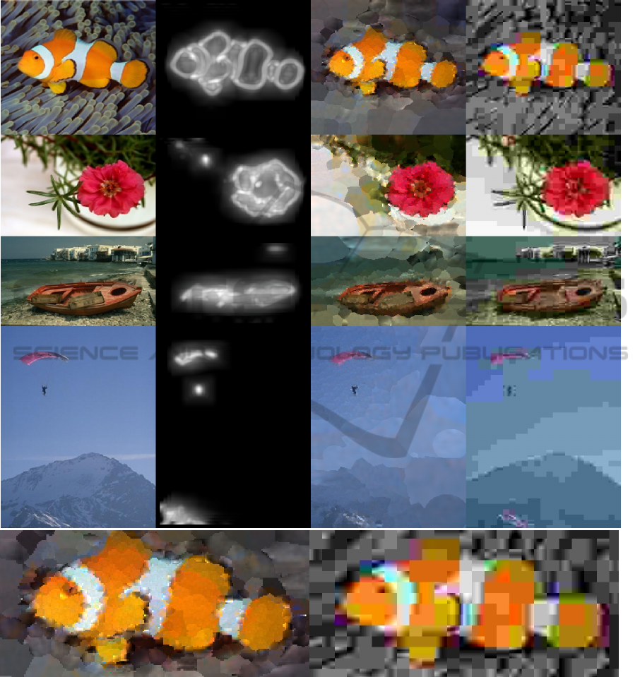
Figure 6: Top in columns: Original color image, saliency map generated for a one or two-color selection (ﬁsh with orange and

white; ﬂower with dark and clear pink; boat with brown; parachute with pink and black), MSIC and JPEG compression for

the test images.Bottom: Fish image detail in both compression methods.

the Earth. In that case, Automatic Building Extraction

from Satellite Imagery algorithms may be used to de-

ﬁne the areas of interest. Then, MSIC may compress

the images keeping higher detail in the built areas. In

a similar way, medical image storage tools might use

MSIC to save images compressed with higher detail

in certain biological tissues or anatomical structures.

Several applications that require image transmis-

sion with low bandwidth may use the algorithm, as

in underwater image transmission, where there are

low data rates compared to terrestrial communication.

Another example of magnitude would be simply the

predicted position of the user’s fovea on the image

in the next frame. This magnitude is useful for ap-

plication in virtual reality glasses, where the image

zone, that is predicted the user is going to focus his

MagnitudeSensitiveImageCompression

379

fovea, will present the highest detail, while surround-

ing zones can be more compressed.

Future work comprises several research lines such

as the use of entropy coding for the information of

each compressed image block, ﬁltering each image

with DCTs, and comparison against other compres-

sion algorithms. Another point to be analysed is the

kind of images used to generate the generic pictorial

codebooks used for compression and restoration, as

the library of training images can be selected for the

chosen task. The test of the algorithm in different

tasks as mentioned in the previous paragraph is a re-

search line that is left for future work too.

ACKNOWLEDGEMENTS

This work is partially supported by Spanish Grant

TIN2010-20177 (MICINN) and FEDER and by the

regional government DGA-FSE.

REFERENCES

Ahmed, N., Natarajan, T., and Rao, K. R. (1974). Discrete

cosine transform. Computers, IEEE Transactions on,

100(1):90–93.

Amerijckx, C., Legat, J.-D., and Verleysen, M. (2003). Im-

age compression using self-organizing maps. Systems

Analysis Modelling Simulation, 43(11):1529–1543.

Cheung, Y. (2005). On rival penalization controlled com-

petitive learning for clustering with automatic cluster

number selection. IEEE Transactions on Knowledge

Data Engineering, (17):1583–1588.

Computer Vision Group, U. o. G. (2002). Dataset

of standard 512x512 grayscale test images.

http://decsai.ugr.es/cvg/CG/base.htm.

Harandi, M. and Gharavi-Alkhansari, M. (2003). Low bi-

trate image compression using self-organized koho-

nen maps. In Proceedings 2003 International Confer-

ence on Image Processing, ICIP’03, volume 3, pages

267–270.

Harel, J., Koch, C., and Perona, P. (2006). Graph-based

visual saliency. In NIPS’06, pages 545–552.

Kohonen, T. (1998). The self-organizing map. Neurocom-

puting, 21(1):1–6.

Laha, A., Pal, N., and Chanda, B. (2004). Design of

vector quantizer for image compression using self-

organizing feature map and surface ﬁtting. Image Pro-

cessing, IEEE Transactions on, 13(10):1291–1303.

Liou, R.J., W. J. (2007). Image compression using sub-band

dct featuresfor self-organizing map system. Journal of

Computer Science and Application, 3(2).

Pelayo, E., Buldain, D., and Orrite, C. (2013). Magni-

tude sensitive competitive learning. Neurocomputing,

112:4–18.

IJCCI2013-InternationalJointConferenceonComputationalIntelligence

380