A Splitting Algorithm for Medical Image Denoising
Ad´erito Ara´ujo
CMUC, Department of Mathematics, University of Coimbra, 3000 Coimbra, Portugal
Keywords:
Finite Differences, Optical Coherence Tomography, Image Denoising.
Abstract:
In this work we consider a stable algorithm for integrating a mathematical model based on mean curvature
motion equation proposed in (Alvarez, Lions, Morel 1992) for image denoising. The scheme is constructed
using a finite difference space discretisation and semi-implicit time discretisation and is considered with a
splitting algorithm that can be implemented in parallel. We apply this algorithm to the problem of denoising
optical coherence tomograms from the human retina while preserving image features.
1 INTRODUCTION
Optical coherence tomography (OCT) is a non-
invasive imaging modality with an increasing number
of applications and it is becoming an essential tool
in ophthalmology allowing in vivo high-resolution
cross-sectional imaging of the retinal tissue. It relies
in certain optical characteristics of light to provide
information of the eye fundus, facilitating the diag-
nosis of several eye pathologies such as macular de-
generation, cone-rod dystrophy, retinopathy and glau-
coma (Junqueira, Carneiro 2005). All these patholo-
gies can be diagnosed more conclusively with the help
OCT(Serranho, Morgado, Bernardes 2012), (Bouma,
Tearney 2002). In fact, previous studies have estab-
lished a link between changes in the blood-retina bar-
rier and in optical properties of the retina (Bernardes,
Santos, Serranho, Lobo, Cunha-Vaz 2011) which can
be identified by this exam.
As any imaging technique that bases its image for-
mation on coherent waves, OCT images suffer from
speckle noise, which reduces its quality. Despeck-
ling optical coherence tomograms from the human
retina is a fundamental step to a better diagnosis or
as a preprocessing stage for retinal layer segmenta-
tion (Bernardes, Maduro, Serranho, Ara´ujo, Barbeiro
Cunha-Vaz 2010). Both of these applications are par-
ticularly important in monitoring the progression of
retinal disorders.
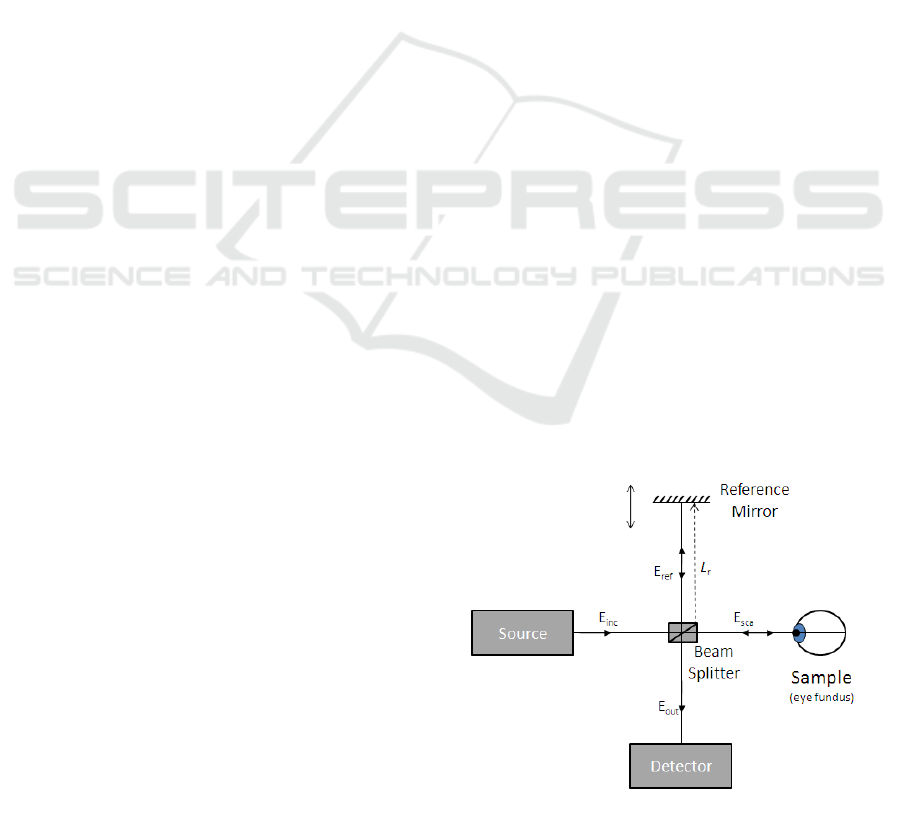
Physically, OCT is based in low coherence inter-
ferometry. This technique uses an electromagnetic
wave with a low coherence length (meaning the wave
is coherent, i.e., highly self-correlated, in a small
space interval). The light beam emitted from the
source is split into two identical beams with a beam
splitter (see Figure 1). Then, while one of the result-
ing waves (i.e. light beam) travels to a reference mir-
ror and back, the other goes to a sample and is re-
flected by structures there present. These reflected
waves recombine at the splitter. The portions of the
waves that are coherent interfere with each other, re-
sulting in an interference pattern which yields infor-
mation about the sample at a given depth (Bernardes,
Cunha-Vaz, Serranho 2012), (Bouma, Tearney 2002).
Figure 1: Schematic of the optical coherence tomography
apparatus.
The main purpose of this work is to consider an
algorithm to reduce the speckle noise for both the vi-
sual assessment and the improved structure segmen-
tation on high- definition spectral domain Cirrus OCT
(Carl Zeiss Meditec, Dublin, CA, USA). This reti-
nal imaging system allows the acquisition of volumes
of 200 × 1024 or 512 × 128 × 1024 voxels, respec-
704
Araújo A..
A Splitting Algorithm for Medical Image Denoising.
DOI: 10.5220/0004634407040709
In Proceedings of the 3rd International Conference on Simulation and Modeling Methodologies, Technologies and Applications (BIOMED-2013), pages
704-709
ISBN: 978-989-8565-69-3
Copyright
c
 2013 SCITEPRESS (Science and Technology Publications, Lda.)

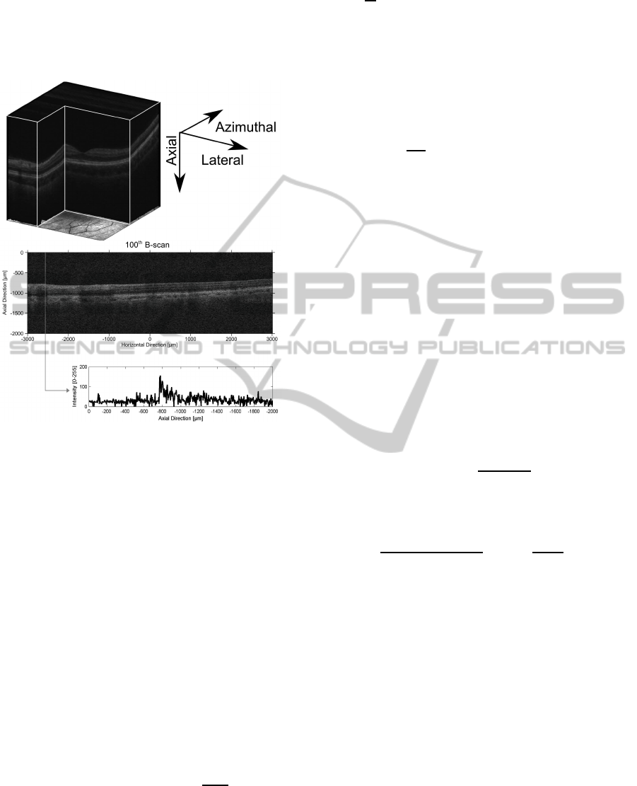
tively, for the lateral, azimuthal and axial directions
(Figure 2). These volumetric data are obtained from a
6000 × 6000 × 2000 µm
3
volume of the human mac-
ula. Additionally, high- resolution B-scan images of
1024× 1024 pixels can be obtained.
Figure 2: Optical coherence tomography (OCT). Top: volu-
metric OCT data shown over an eye fundus reference. Bot-
tom example of a B-scan (top) and an A-scan profile (bot-
tom).
The paper is organised as follows. In Section 2 we
present the mathematical model for image denoising.
In Section 3 we define the finite difference implicit-
explicit scheme that can be implemented in parallel
and prove that the algorithm is stable with respect to
the infinity norm. In Section 3 we consider the appli-
cation of the proposed filter to an example with syn-
thetic as well as to an OCT high-resolution B-scan
from the human eye fundus. We finish with some con-
clusions.
2 MATHEMATICAL MODEL
Let φ ∈ C
2
(Ω× [0,T]) with Ω ⊂ R
2
a compact set and
φ
0
∈ C(Ω). We consider the problem

















φ
t
= g(|∇G
σ
∗ φ|)|∇φ|div

∇φ
|∇φ|

,
(x,y) ∈ Ω, t ∈]0,T]
φ(x,y, 0) = φ
0
(x), (x,y) ∈ Ω
φ(x,y,t) = 0, (x,y) ∈ ∂Ω, t ∈ [0,T]
(1)
where
∂φ
∂ν
denotes the derivative in the direction of
the exterior normal to ∂Ω, G
σ
a smoothing kernel
that depends on a parameter σ (e.g. a Gaussian) and
g(s) is a nondecreasing real function which tends to
zero as s → ∞. This problem was proposed in (Al-
varez, Lions, Morel 1992) for image smooting and
edge detection where φ
0
(x,y) represents the try level
of the original noisy image, φ(x, y,t) is its smoothed
version depending on the scale parameter t. The
term |∇φ|div

∇φ
|∇φ|

represents a degenerate diffusion
term, which diffuses φ in the direction to its gradient.
The term g(|∇G
σ
∗ φ|) is used for the enhancement to
the edges, since it controls the speed of the diffusion:
if the gradient of φ has a small mean in a neighbour-
hood of a point, this point is considered the interior
point of a smooth region of the image and the diffu-
sion is strong; if the gradient has a large mean value
on the neighbourhood of a point, this point is consid-
ered an edge point and the diffusion spread is lowered
since g(s) is small for large s.
The equation (1) is difficult to study since, besides
its non-linearity, is not defined in the points where
|∇φ| = 0. In order to prevent the situation of possi-
ble zero gradients, we will consider the Evans-Spruck
type regularization (Evans, J. Spruck 1991) and con-
sider |∇
ε
φ| instead of |∇φ|, where
∇
ε
φ = (∇
T
φ,ε)
T
,
with 0 ≤ ε ≪ 1. In other words, we replace |∇φ| by
|∇
ε
φ| =
q
|∇φ| + ε
2
in (1) obtaining the modified problem that we will
write in the form

















φ
t
g(|∇G
σ
∗ φ|)|∇
ε
φ|
= div

∇φ
|∇
ε
φ|

,
(x,y) ∈ Ω, t ∈]0, T]
φ(x,y, 0) = φ
0
(x), (x,y) ∈ Ω
φ(x,y,t) = 0, (x,y) ∈ ∂Ω, t ∈ [0,T]
(2)
Note that, for zero gradients, this problem reduces
to the heat equation, which is suitable for smoothing
purposes. On the other hand, for large values of the
gradient, the influence of ε can be neglected.
3 MUMERICAL METHOD
3.1 A Linearly Implicit Finite
Difference Scheme
Let ∆t > 0 and t
n
= n∆t, with n = 0,...,N such that
t
0
= 0 and t
N
= T and Ω =]0,X[×]0,Y[, N
x
,N
y
∈ N
ASplittingAlgorithmforMedicalImageDenoising
705

and h > 0 such that
h =
X
N
x
=
Y
N
y
.
Let us also consider x
i
= ih and y
j
= jh, for i =
0,1, ...,N
x
and j = 0,1, ...,N
y
. These points define a
rectangular grid that we denote by
Ω
h
= {(x
i
,y
j
) : i = 0,1, ...,N
x
, j = 0,1, ...,N
y
}.
Let φ
n
ij
≈ φ(x
i
,y
j
,n∆t) denote the solution of the finite
differences problem
1
g
n
ij
|∇
ε,h
φ
n
ij
|
φ
n+1
ij
− φ
n
ij
∆t
= D
+
x
D
−
x
φ
n+1
ij
|∇
ε,h
φ
n
ij
|
!
+D
+
y
D
−
y
φ
n+1
ij
|∇
ε,h
φ
n
ij
|
!
, (3)
in which
g
n
ij
= g(|∇G
σ
∗ φ
n
ij
|),
∇
ε
φ =

D
−
x
φ
n
ij
,D
−
y
φ
n
ij
,ε

T
,
and
|∇
ε,h
φ
n
ij
| =
q
(D
−
x
φ
n
ij
)
2
+ (D
−
y
φ
n
ij
)
2
+ ε
2
,
with the first order finite differences operators defined
by
D
−
x
U
ij
=
U
ij
−U
i−1, j
h
,i = 1, ...,N
x
, j = 1, ...,N
y
− 1,
D
+
x
U
ij
=
U
i+1, j
−U
ij
h
,i = 0, ...,N
x
− 1, j = 1,...,N
y
− 1,
D
−
y
U
ij
=
U
ij
−U
i, j−1
h
,i = 1, ...,N
x
− 1, j = 1,...,N
y
,
D
+
y
U
ij
=
U
i, j+1
−U
ij
h
,i = 1, ...,N
x
− 1, j = 0,...,N
y
− 1.
3.2 A Splitting Algorithm
The main idea behind splitting algorithms is to split
the problem we want to solve in several simpler sub-
problems, independent or not, conveniently chosen.
Let S be a space of functions and A an operator
defined on S. Let us consider the equation
∂φ
∂t
= A (t,φ) + f(t) in Ω×]0,T], φ(0) = φ
0
∈ S.
Let us now suppose that A and f can be decom-
posed in the following way
A = A
1
+ ··· + A
m
and f = f
1
+ ··· + f
m
.
Splitting algorithms take advantage of this decompo-
sition, considering the m subproblems
∂φ
∂t
= A
k
(t,φ) + f
k
(t) in Ω×]0,T], k = 1,..., m.
Considering the time step ∆t, t
n
= n∆t, for n =
1,...,N, and φ
n
= φ(x,t
n
), with φ
0
= φ
0
, in (Lu, Neit-
taanmaki, Tai 1992) the authors proposed the follow-
ing parallel algorithm:
At each level time n = 0,..., N − 1 compute:
1.
φ
n+
k
2m
− φ
n
m∆t
= A
k
φ
n+
k
2m
+ f
k

(n+
1
2
)∆t

,
k = 1,... ,m;
2. φ
n+1
=
1
m
m
∑
k=1
φ
n+
k
2m
.
We pretend to consider the same approach to de-
fine a splitting algorithm for the discretized equation
(3). Let us consider A = A
1
+ A
2
with:
A
1
(φ
n+1
) = D
+
x
D
−
x
φ
n+1
ij
|∇
ε,h
φ
n
ij
|
!
and
A
2
(φ
n+1
) = D
+
y
D
−
y
φ
n+1
ij
|∇
ε,h
φ
n
ij
|
!
.
We may then define the following sub-equations
1
g
n
ij
|∇
ε,h
φ
n
ij
|
φ
n+
1
4
ij
− φ
n
ij
2∆t
= A
1
(φ
n+1
)
and
1
g
n
ij
|∇
ε,h
φ
n
ij
|
φ
n+
1
4
ij
− φ
n
ij
2∆t
= A
2
(φ
n+1
).
Let us consider the first equation written in the
form
1
g
n
ij
|∇
ε,h
φ
n
ij
|
φ
n+
1
4
ij
− φ
n
ij
2∆t
=
φ
n+
1
4
i−1, j
h
2
|∇
ε,h
φ
n
i, j
|
−
2
h
2
φ
n+
1
4
ij
1
|∇
ε,h
φ
n
i+1, j
|
+
1
|∇
ε,h
φ
n
i, j
|
!
+
φ
n+
1
4
i+1, j
h
2
|∇
ε,h
φ
n
i+1, j
|
. (4)
Let Φ
n
the (N
y
− 1)(N
x
− 1)-dimensional vector
Φ
n
=

φ
n
1,1
, .. . , φ
n
N
x
−1,1
, ... , φ
n
1, j
, ... , φ
n
N
x
−1, j
,
... , φ
n
1,N
y
−1
, .. ., φ
n
N
x
−1,N
y
−1
i
T
and A
1
the (N
y
−1)(N
x
−1) ×(N
y
−1)(N
x
−1) matrix
with (N
y
−1) blocks of (N
x
−1)×(N
x
−1) tridiagonal
matrices. The j-th block of A
1
, j = 1,..., N
y
− 1, has
entries
a
i,i−1
=
g
n
ij
h
2
,
SIMULTECH2013-3rdInternationalConferenceonSimulationandModelingMethodologies,Technologiesand
Applications
706

a
i,i
= −
2g
n
ij
h
2
|∇
ε,h
φ
n
i, j
|
|∇
ε,h
φ
n
i+1, j
|
+ 1
!
,
a
i,i+1
=
g
n
ij
|∇
ε,h
φ
n
i, j
|
h
2
|∇
ε,h
φ
n
i+1, j
|
,
for i = 1,...,N
x
− 1.
Then, the first sub-equation may be written in the
form
Φ
n+
1
4
− Φ
n
2∆t
= A
1
Φ
n+
1
4
.
Following the same approach, we conclude that
the second sub-equation is equivalent to
Φ
n+
1
2
− Φ
n
2∆t
= A
2
Φ
n+
1
2
,
where A
2
is a matrix of the same type as A
1
with en-
tries
a
k,k−(N
y
−1)
=
g
n
ij
h
2
,
a
k,k
= −
2g
n
ij
h
2
|∇
ε,h
φ
n
i, j
|
|∇
ε,h
φ
n
i, j+1
|
+ 1
!
,
a
k,k+(N
y
−1)
=
g
n
ij
|∇
ε,h
φ
n
i, j
|
h
2
|∇
ε,h
φ
n
i, j+1
|
,
where k is related with i, j by k = ( j − 1)(N
x
− 1) + i.
Since both A
1
and A
2
strictly diagonal dominant
matrices, they are invertible and then we may define
the following algorithm to solve (2) numerically:
At each level time n = 0,..., N − 1 compute:
1. Compute, for i = 1,..., N
x
−1 and j = 1,...,N
y
−1,
|∇
ε,h
φ
n
ij
| =
q
(D
−
x
φ
n
ij
)
2
+ (D
−
y
φ
n
ij
)
2
+ ε
2
;
2. Construct A
1
and A
2
;
3. Solve
(I − 2∆tA
1
)φ
n+
1
4
= φ
n
and
(I − 2∆tA
2
)φ
n+
1
2
= φ
n
;
4. φ
n+1
=
φ
n+
1
4
+ φ
n+
1
2
2
.
With the properties of the matrices A
1
and A
2
we
may prove that the algorithm is stable for the k.k
∞
norm. In fact, according to





1+
4∆tg
n
ij
h
2
|∇
ε,h
φ
n
i, j
|
|∇
ε,h
φ
n
i+1, j
|
+ 1
!





<




−
2∆tg
n
ij
h
2




+





−
2∆tg
n
ij
|∇
ε,h
φ
n
i, j
|
h
2
|∇
ε,h
φ
n
i+1, j
|





,
the matrix I − 2∆tA
1
is strictly diagonal dominant.
Since the diagonal entries of I − 2∆tA
1
are positive
and the other entries are non-positive, we conclude
that I − 2∆tA
1
is an M-matrix. In the same way, we
conclude that I − 2∆tA
2
is also an M-matrix. Then
there exists two positive constantsC
1
and C
2
such that
k(I − 2∆tA
i
)
−1
k
∞
≤ C
i
, i = 1, 2.
Then kΦ
n+
1
4
k
∞
+ kΦ
n+
1
2
k
∞
≤ (C
1
+ C
2
)kφ
n
k
∞
and therefore
kΦ
n+1
k
∞
≤ 2

k(Φ
n+
1
4
k
∞
+ kΦ
n+
1
2
)k
∞

≤ 2(c
1
+ c
2
)kφ
n
k
∞
,
which proves the stability.
4 NUMERICAL RESULTS
In this section, we report our numerical testing for the
proposed algorithm. In the Example 1, the basic fea-
tures of the algorithm are explained. The second ex-
ample is a two dimensional OCT image. In both ex-
amples we consider
g(s) =
1
1+ s
2
and
G
σ
(x,y) = σ
−1/2
exp(−|x
2
+ y
2
|/(4σ)).
Other choices for the function g may be found in lit-
erature but this is the most commonly used in practi-
cal applications (Didas, Weickert 2007), (Plonka, Ma
2008).
For the proposed filter we consider a diffusion
time of 0.3 s. The filter was applied using 10 itera-
tions with a time step ∆t = 0.03 s. The parameters
for the gaussian kernel was σ = 1.5. We also consider
the spatial step size h = 1 and the relaxation parameter
ε = 10
−5
. The parameter ε can be tuned in each appli-
cation but it has no influence in the overall behavior
of the algorithm.
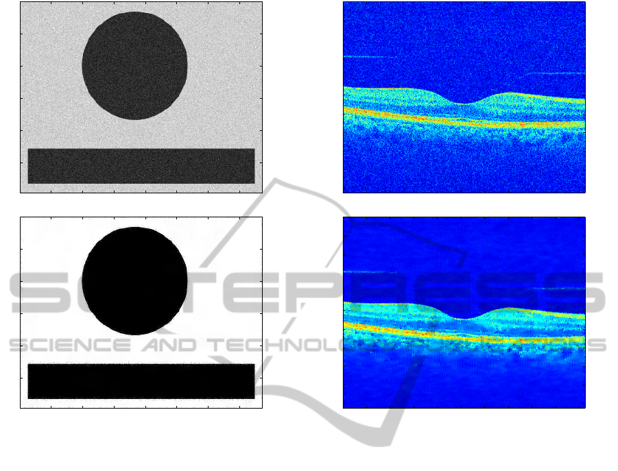
Example 1. For our first test, we use the image
shown in Figure 3. This image was obtained from
a binary image by introducing 40% of salt and pep-
per noise. Salt and pepper noise presents a serious
problem for segmentation algorithms that use image
gradient information. This example, and others made
with synthetic data, show that the algorithm preserves
contrasts in the original image.
ASplittingAlgorithmforMedicalImageDenoising
707

50 100 150 200 250 300 350
50
100
150
200
250
50 100 150 200 250 300 350
50
100
150
200
250
Figure 3: Top: Original test noisy image; bottom: denoised
image.
Example 2. We consider a data set of images given
by the Institute of Biomedical Research in Light and
Image (IBILI), a research department of the Faculty
of Medicine of the University of Coimbra, that cor-
respond to real human eye fundus OCT data using
the high-definition spectral domain Cirrus OCT (Carl
Zeiss Meditec, Dublin, CA, USA). In our numeri-
cal tests, we considered 32 B-scans using the mac-
ular cube protocol from 32 eye fundus scans from 13
healthy volunteers, 3 eyes with choroidal neovascu-
larization, 2 with cystoid macular edema, 9 with dia-
betic retinopathy and 5 with age-related macular de-
generation. In Figure 4 we just present one of these
tests for a randomly chosen image.
Note the well-defined interface between the tissue
and the vitreous regions. This allows us to conclude
that the algorithm can be used not only to improve
visual assessments of medical images but also as a
preprocessor for image segmentation.
50 100 150 200 250 300 350 400 450 500
100
200
300
400
500
600
700
800
900
1000
50 100 150 200 250 300 350 400 450 500
100
200
300
400
500
600
700
800
900
1000
Figure 4: Top: Original OCT noisy image; bottom: de-
noised image.
5 CONCLUSIONS
AND FUTURE WORK
In this work we consider an algorithm for integrat-
ing a mathematical model based on mean curvature
motion equation proposed in (Alvarez, Lions, Morel
1992) for image denoising. The scheme has good sta-
bility properties and can be implemented in parallel.
The application to despeckling optical coherence to-
mograms from the human retina show that the algo-
rithm can be used as a preprocessing stage for OCT
retina layer segmentation.
In the near future work we want to use well-
known speckle-reduction performance metrics (Sali-
nas, Fern´andez 2007) to compare this algoritm with
other filters, in particular with the nonlinear complex
diffusion filter considered in (Bernardes, Maduro,
Serranho, Ara´ujo, Barbeiro Cunha-Vaz 2010). In ad-
dition to this particular area of application in the fun-
dus of the human eye, this filter may be applied as
well to different data sources corrupted with speckle
noise, such as medical ultrasound.
SIMULTECH2013-3rdInternationalConferenceonSimulationandModelingMethodologies,Technologiesand
Applications
708

ACKNOWLEDGEMENTS
This work has been partially supported by Centro de
Matem´atica da Universidade de Coimbra (CMUC),
funded by the European Regional Development
Fund through the program COMPETE and by the
Portuguese Government through the FCT - Fundac¸˜ao
para a Ciˆencia e a Tecnologia under the project
PEst-C/MAT/UI0324/2011, and by FCT under the
project PTDC/SAU-ENB/119132/2010) and COM-
PETE (QREN-FCOMP-01-0124-FEDER-021014)
program. The author was also partially supported by
program the project UTAustin/MAT/0066/2008.
REFERENCES
L. Alvarez, P-L Lions and J-M Morel (1992). Image Se-
lective Smoothing and Edge Detection by Nonlinear
Diffusion II. SIAM Journal on Numerical Analysis,
29(3), 845–866.
R. Bernardes, C. Maduro, P. Serranho, A. Ara´ujo, S. Bar-
beiro, and J. Cunha-Vaz (2010). Improved adaptive
complex diffusion despeckling filter. Optics Express,
18(23), 24048–24059.
R. Bernardes, T. Santos, P. Serranho, C. Lobo, and J.
Cunha-Vaz (2011), Noninvasive evaluation of retinal
leakage using OCT, Ophtalmologica, 226(2), 29–36.
R. Bernardes, J. Cunha-Vaz, and P. Serranho (2012). Op-
tical Coherence Tomography: a Concept Review. In
Biological and Medical Physics. R. Bernardes and J.
Cunha-Vaz, Eds. Berlin, Heidelberg: Springer Berlin
Heidelberg.
B. Bouma and G. Tearney (2002), Handbook of optical
coherence tomography. Marcel Dekker, New York.
S. Didas and J. Weickert (2007), Combining curvature mo-
tion and edge-preserving denoising scale space and
variational methods in computer vision, Lecture Notes
in Computer Science, 4485, 568–579.
L. C. Evans and J. Spruck (1991). Motion of level sets by
mean curvature I. J. Differential Geometry, 33, 635–
681.
L. Junqueira and J. Carneiro (2005), Basic Histology: Text
& Atlas (Junqueira’s Basic Histology). McGraw-Hill
Medical.
T. Lu, P. Neittaanmaki, and X.-C. Tai (1992). A parallel
splitting up method for partial differential equations
and its application to Navier-Stokes equation. RAIRO
Math. Model. and Numer. Anal., 26, 673–708.
G. Plonka and J. Ma (2008), Nonlinear regularized reaction-
diffusion filters for denoising of images with textures,
IEEE Trans. Image Process, 17(8), 1283–1294.
H. M. Salinas, and D. C. Fern´andez (2007) Comparison
of PDE-based nonlinear diffusion approaches for im-
age enhancement and denoising in optical coherence
tomography, IEEE Trans. Med. Imaging, 26(6), 761–
771.
P. Serranho, M. Morgado and R. Bernardes (2012) Optical
Coherence Tomography: a concept review. In Opti-
cal Coherence Tomography: A Clinical and Technical
Update. R. Bernardes & J. Cunha-Vaz Eds., Springer-
Verlag, 139–156.
ASplittingAlgorithmforMedicalImageDenoising
709