
A Recursive Approach For Multiclass Support Vector Machine
Application to Automatic Classification of Endomicroscopic Videos
Alexis Zubiolo
1
, Gr
´
egoire Malandain
1
, Barbara Andr
´
e
2
and
´
Eric Debreuve
1
1
Team Morpheme (Lab I3S/Inria SA-M/iBV), University of Nice-Sophia Antipolis/CNRS/Inria, Sophia Antipolis, France
2
Mauna Kea Technologies, 9 rue d’Enghien, 75010 Paris, France
Keywords:
Multiclass classification, Supervised Learning, Hierarchical Approach, Graph Minimum-cut, Support Vector
Machine (SVM).
Abstract:
The two classical steps of image or video classification are: image signature extraction and assignment of a
class based on this image signature. The class assignment rule can be learned from a training set composed
of sample images manually classified by experts. This is known as supervised statistical learning. The well-
known Support Vector Machine (SVM) learning method was designed for two classes. Among the proposed
extensions to multiclass (three classes or more), the one-versus-one and one-versus-all approaches are the most
popular ones. This work presents an alternative approach to extending the original SVM method to multiclass.
A tree of SVMs is built using a recursive learning strategy, achieving a linear worst-case complexity in terms
of number of classes for classification. During learning, at each node of the tree, a bi-partition of the current
set of classes is determined to optimally separate the current classification problem into two sub-problems.
Rather than relying on an exhaustive search among all possible subsets of classes, the partition is obtained by
building a graph representing the current problem and looking for a minimum cut of it. The proposed method
is applied to classification of endomicroscopic videos and compared to classical multiclass approaches.
1 INTRODUCTION
The problem of automatic image (or video, or object)
classification is to find a function that maps an im-
age to a class or category among a number of pre-
defined classes. An image can be viewed as a vec-
tor of high-dimension. In practice, it is preferable
to deal with a synthetic signature of lower dimen-
sion. Therefore, the two classical steps of image clas-
sification are: image signature extraction (Oliva and
Torralba, 2001) and signature-based image classifica-
tion (Cortes and Vapnik, 1995). (Note that the signa-
ture extraction step can itself be the result of a learn-
ing process (Sivic and Zisserman, 2003).) The clas-
sification rule can be learned from a set of training
sample images manually classified by experts. This
is known as supervised statistical learning where sta-
tistical refers to the use of samples and supervised
refers to the sample classes being provided. In this
paper, we are interested in the learning aspect of the
multiclass
1
problem when using a binary classifica-
tion approach as a building block. The Support Vec-
1
Traditionally in classification, multiclass means “three
classes or more” while the two-class case is referred to as
binary classification.
tor Machine (SVM) (Cortes and Vapnik, 1995) is a
well-known binary classifier that will be used in the
following. In its original, linear version, it makes it
possible to separate two sets of d-dimensional sam-
ples (the training sample signatures for two classes)
by finding a particular hyperplane, i.e., by determin-
ing its two parameters b ∈ R and w ∈ R
d
. It does
so by maximizing the half-margin 1/
k
w
k
which rep-
resents the distance to the nearest training sample of
any class. Whenever the two classes are not linearly
separable, the soft margin strategy can be used to ac-
count for misclassifications and the kernel trick can be
applied to extend the SVM method to nonlinear sep-
aration (Scholkopf and Smola, 2001). The parameter
tuning the soft margin tolerance is usually denoted by
C (see Fig. 3).
Among the proposed extensions of binary clas-
sification methods (such as the SVM) to multiclass
(three classes or more), the one-versus-one and one-
versus-all approaches are the most popular ones. Let
us suppose that there are p ≥ 3 classes. The idea
of the one-versus-all strategy is to oppose to any of
the classes the union of the remaining p − 1 classes.
Then, p SVM classifiers are determined, each one
441
Zubiolo A., Malandain G., André B. and Debreuve É..
A Recursive Approach For Multiclass Support Vector Machine - Application to Automatic Classification of Endomicroscopic Videos.
DOI: 10.5220/0004654704410447
In Proceedings of the 9th International Conference on Computer Vision Theory and Applications (VISAPP-2014), pages 441-447
ISBN: 978-989-758-003-1
Copyright
c
2014 SCITEPRESS (Science and Technology Publications, Lda.)

scoring, say, positively for one of the classes. To clas-
sify a new image, its signature is tested against all the
SVMs and it is assigned to the class with the high-
est score (largest distance to the SVM hyperplane).
The one-versus-one strategy opposes the classes by
pair for all possible pairs. Therefore,
p(p−1)
2
SVMs
are determined. For classification, a new image sig-
nature is tested against all the SVMs, each SVM
votes in favor of one of the two classes it corresponds
to, and the image is assigned to the highest voted
class. Other methods also learn all the pairwise SVMs
(as for one-versus-one) but use a different scheme
to predict the class during the classification step. It
is the case for the Decision Directed Acyclic Graph
(DDAG (Platt et al., 2000)) and the Adaptive Directed
Acyclic Graph (ADAG (Kijsirikul et al., 2002)) meth-
ods.
As an alternative to these aforementioned strate-
gies, hierarchical methods can be designed. For ex-
ample, the work done in (Tibshirani and Hastie, 2006)
applies clustering techniques to the different classes
and considers the widths of the one-versus-one SVM
margins to define linkage criteria. This paper presents
a recursive learning strategy to extend a binary classi-
fication method to multiclass. A tree of SVMs is built
using a recursive learning strategy in such a way that
a linear worst-case complexity is achieved for clas-
sification. During learning, at each node of the tree,
a bi-partition of the set of classes is found to deter-
mine an optimal separation of the current classifica-
tion problem into two sub-problems. This decision re-
lies on building a graph representing the current prob-
lem and looking for a minimum cut of it. The pro-
posed method is applied to classification of endomi-
croscopic videos and compared to classical multiclass
approaches.
2 WHY A RECURSIVE
STRATEGY?
2.1 Motivations
When learning is performed offline (as described
in the present context), it is interesting to design a
method with a low classification complexity, even if
we have to pay the price of a high learning complex-
ity for it. The classification complexities (in terms of
number of classes) of the one-versus-one and the one-
versus-all strategies are quadratic and linear, respec-
tively. When thinking about a complexity lower than
linear, the logarithmic one comes to mind. Recur-
sive (or, equivalently, hierarchical) approaches natu-
rally lead to such performances. Hence, we propose
to decompose the original multiclass problem with p
classes into two sub-problems (of “similar size”, ide-
ally), i.e., involving q
1
and q
2
classes, respectively,
with q
1
+ q
2
= p. Let us denote by virtual class the
union of classes involved in a sub-problem. Decid-
ing which virtual class a given signature belongs to is
a classical binary classification. Then, as long as the
sub-problems involve three classes or more, they can
be further decomposed into smaller sub-problems.
The question is thus to optimally decompose a given
p-class problem, p ≥ 3, into two sub-problems (see
Section 3.1).
Another motivation for such a recursive approach
is the fair balance between the sub-problems. In-
deed, as already mentioned, the two virtual classes
resulting from the decomposition of a p-class prob-
lem should each gather the same (or almost the same)
number of classes, ideally. If all the classes have
roughly the same number of training signatures, so
will have the virtual classes. It is certainly desirable
for the determination of a reliable binary classification
rule, as opposed to the case where one virtual class
contains much less samples than the other one. This
fair balance property also holds for the one-versus-
one strategy (unfortunately, as already mentioned, it
has a quadratic classification complexity). However,
it does not for the one-versus-all strategy which relies
on virtual classes gathering either one class or p − 1
classes.
Finally, with the proposed recursive approach, the
successive binary classifications into virtual classes
progressively narrow the classification decision down
to the assignment of a unique label among the prede-
fined classes. The one-versus-one and one-versus-all
approaches do not exhibit such a coherence since sev-
eral predefined classes can receive votes when test-
ing a signature against the different SVMs. The final
classification decision must deal with competing par-
tial decisions. Although the practical solutions
2
make
sense, the principle is not fully satisfying. With the
one-versus-one strategy, for a signature belonging to,
say, class i, it can be further noted that all the SMVs
learned to distinguish between class j and class k,
j 6= i and k 6= i, will be used to decide whether the sig-
nature belongs to class j or class k, and these uninfor-
mative partial decisions will be accounted for in the
final decision. This is know as the non-competence
problem.
2
Maximum number of votes for one-versus-one or max-
imum positive score for one-versus-all.
VISAPP2014-InternationalConferenceonComputerVisionTheoryandApplications
442

2.2 Optimizing the Classification
Complexity Alone
Let us suppose that there are p ≥ 3 predefined classes.
Let us recall that a q-subset is a set containing q ele-
ments taken from a larger set containing p elements.
Let us remind that the number of q-subsets is given
by the binomial coefficient
p
q
.
As mentioned in Section 2.1, the general idea
is to decompose a p-class problem into a q
1
-class
sub-problem and a q
2
-class sub-problem where q
1
+
q
2
= p, and continuing recursively with the two sub-
problems. Each decomposition relies on a binary
classifier separating q
1
classes for the q
2
other ones.
Thus, a tree of binary classifier is built. For classifi-
cation, this tree has to be traversed from the root to a
leaf, following a branch depending on the responses
of the node classifiers. To optimize the classifica-
tion complexity in terms of the number of classifiers
that are tested, the tree must be of minimal depth or,
equivalently, as close as possible to a perfect binary
tree. This is achieved by enforcing the following con-
straints:
q
1
+ q
2
= p (partition constraint)
|q
1
− q
2
| ≤ 1 (balance constraint)
. (1)
The classification complexity is then equal to the tree
depth, i.e. log
2
(p). However, the limiting factor of
such an approach is the combinatorial learning com-
plexity in terms of the number of binary classifiers
that must be determined at each node of the tree. Sec-
tion 3 proposes another strategy involving graph the-
ory in order to overcome this issue.
3 PROPOSED METHOD: GRAPH
CUT BASED SVM TREE
(GC-SVM)
3.1 Trade-off between Learning and
Classification Complexities
The following description is valid for any binary clas-
sifier framework. However, this paper focuses on the
SVM example. First, similarly to the one-versus-
one approach, we compute the SVMs between each
pair of classes among the p ≥ 3 predefined classes.
Now, following the recursive strategy described in
Sections 2.2 and 2.1, let us assume that we are about
to deal with a node containing more than three classes
(originally, the root node contains all p classes).
The idea is to use graph theory tools to determine
a bi-partition of this set of classes. This bi-partition
will not necessarily be balanced (i.e. the second con-
dition of Eq. 1 will no longer be taken into account).
A labeled, weighted, undirected, complete graph G is
built such that:
• Each node represents a class (i.e., node i ≡ class
i);
• The weight c
i j
of the edge linking nodes i and
j is equal to the inverse of the margin of the
SVM computed between classes i and j, i.e., c
i j
=
w
i j
2
.
The minimum cut of G will result in a bi-partition
of the nodes such that the sum of the weights of
the edges cut is minimal. It is computed using
Stoer-Wagner’s min-cut algorithm (Stoer and Wag-
ner, 1997). Thanks to the chosen graph definition,
this will also correspond to separating the classes of
pairs that have a large SVM margin. Hence, the two
virtual classes, union of the classes on each side of the
partition, will tend to have a large margin too. We just
have to compute the corresponding SVM and assign
it to the current node. Therefore, for the whole tree
building, p(p − 1)/2 SVMs are computed first, then
additional SVMs are computed for each non-leaf tree
node. There are p − 1 such nodes. Actually, for the
nodes that are parents of two leaves, the SVM needs
not be computed since it corresponds to one of the
SVMs first computed for each pair of classes. There-
fore, there are at most p − 1 additional SVMs to be
computed. As a result, O(p
2
) SVMs are computed in
total. The proposed learning method is described in
algorithm 1. It calls the procedure MINCUT which is
entirely defined in (Stoer and Wagner, 1997).
Once the tree T of SVMs and virtual classes has
been built, the classification of a new image signature
is simply performed by following a unique branch
based on the successive decisions of the nodes’
SVMs. The branch leaf contains the label of the iden-
tified predefined class. Figure 1 presents an instance
of SVM tree for five classes labeled 1 to 5.
{1, 2, 4}, {3, 5}, SVM
1
{1, 4}, {2}, SVM
2a
{1}, {4}, SVM
3
1 4
2
{3}, {5}, SVM
2b
3 5
Figure 1: Type of tree that the proposed method builds dur-
ing the learning stage. An example of classification of a
new image signature is also illustrated by showing the vis-
ited nodes in boldface (read from root to leaf).
ARecursiveApproachForMulticlassSupportVectorMachine-ApplicationtoAutomaticClassificationof
EndomicroscopicVideos
443

Algorithm 1: The GC-SVM algorithm.
1: procedure GCSVM(L, p)
2: T ← empty tree
3: if p == 1 then
4: Create a node with label l
1
and add it to T
5: else if p == 2 then
6: Create two nodes with labels l
1
and l
2
and
add them to T
7: else
8: a ← an arbitrary node of G
9: (L
1
,L
2
) = MINCUT(G,a)
10: p
1
← the number of classes in L
1
11: p
2
← the number of classes in L
2
12: T
1
= GCSVM(L
1
, p
1
)
13: T
2
= GCSVM(L
2
, p
2
)
14: let T
1
be the left child of T
15: let T
2
be the right child of T
16: end if
17: return T
18: end procedure
3.2 Complexity
Let us start with the learning step.
Proposition 1. The number of SVM computed during
the learning step is O(p
2
).
Proof. The number of SVM computed is equal to the
sum of:
• The number of binary SVM we compute to build
the graph O(p
2
),
• The number of nodes in the graph built, i.e. O(p).
As a result, the total number of SVM computed is
O(p
2
).
As for the classification step, the number of SVM
used depends on the way the binary tree is built: it
is equal to the depth of the tree. This is the reason
why we distinguish the worst-case complexity and the
best-case complexity.
Proposition 2 (Worst-case complexity for classifica-
tion step). The worst-case complexity for the classifi-
cation step is O(p).
Proof. The worst-case scenario happens when the
tree built is a degenerate tree, i.e. when for each par-
ent node, there is only one associated child node. In
this case, the depth of the tree is O(p). So is the com-
plexity.
Proposition 3 (Best-case complexity for classifica-
tion step). The best-case complexity for the classifi-
cation step is O(log(p)).
Proof. The best-case happens when the tree is bal-
anced, i.e. when for each parent node, there are two
associated child nodes whenever it is possible. In such
a case, the depth is logarithmic, and as a result the
complexity is O(log(p)).
Let us compare the methods above-mentionned
with the most commonly used algorithms. Table 1
presents the complexities in terms of number of
classes for both learning (offline task performed only
once) and classification (performed on-demand), for
one-versus-one, one-versus-all, the Directed Acyclic
Graph SVM method (DAGSVM) (Platt et al., 2000),
and the proposed methods.
The proposed method offers a lower classification
complexity and still a reasonable learning complex-
ity. Moreover, since testing a decomposition means
learning a binary classifier, and since the computer
time needed for a learning depends on the number
of training samples, a straightforward way to reduce
the learning time is to subsample cleverly the training
set (Bakir et al., 2005).
4 EXPERIMENTAL RESULTS
The proposed method has been implemented in Mat-
lab using the SVM-KM (Support Vector Machine and
Kernel Methods) toolbox (Canu et al., 2005) which
implements the binary SVM classifier as well as the
one-versus-one and one-versus-all strategies. It has
been applied to automatic classification of endomi-
croscopic videos.
The medical database to which we apply the
classification methods contains 116 endomicroscopic
videos, each of them showing a colonic polyp in vivo
at the cellular level. These videos were acquired at the
Mayo Clinic in Jacksonville during endoscopy proce-
dures on 65 patients, using a technology called probe-
based Confocal Laser Endomicroscopy (pCLE) de-
veloped by Mauna Kea Technologies. Each video is
assigned to a pathological class which is the histo-
logical diagnosis established by an expert pathologist
from a biopsy on the imaged polyp. The 5 patho-
logical classes are: purely benign (14 videos), hy-
perplastic (21 videos), tubular adenoma (62 videos),
tubulovillous adenoma (15 videos) and adenocarci-
noma (4 videos) (See Fig. 2). In (Andr
´
e et al., 2011),
a bag-of-visual-words method was proposed to build
the visual signatures of these videos, based on mosaic
images associated with stable video subsequences. To
VISAPP2014-InternationalConferenceonComputerVisionTheoryandApplications
444
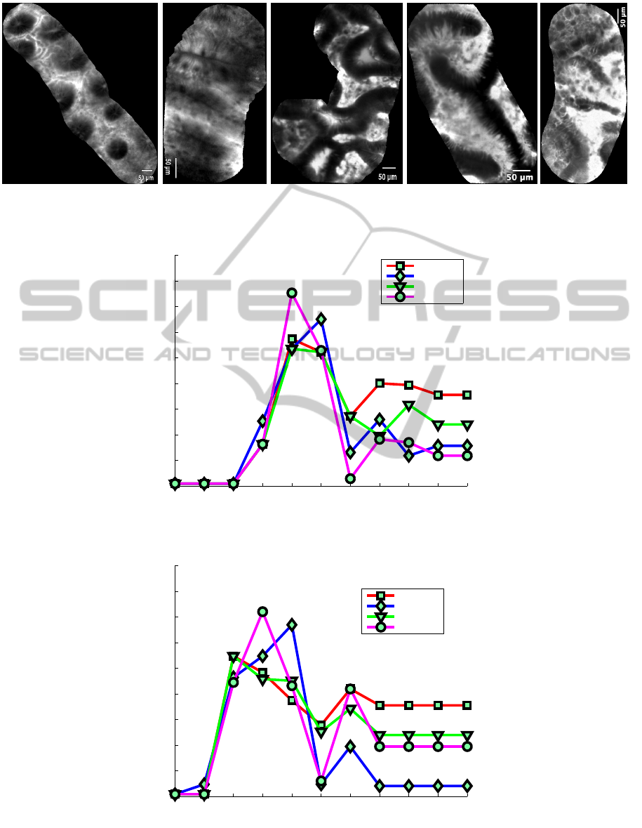
Purely benign Hyperplastic Tubular adenoma Tubulovillous adenoma
Adenocarcinoma
Figure 2: Examples of annotated endomicroscopic videos.
0 2 4 6 8 10 12 14 16 18 20
0.52
0.54
0.56
0.58
0.6
0.62
0.64
0.66
0.68
0.7
log
2
C
accuracy
One vs. One
One vs. All
DAGSVM
GC−SVM
(a) Gaussian radial basis function kernel : k(x
i
,x
j
) = exp
x
i
− x
j
2
0 2 4 6 8 10 12 14 16 18 20
0.52
0.54
0.56
0.58
0.6
0.62
0.64
0.66
0.68
0.7
log
2
C
accuracy
One vs. One
One vs. All
DAGSVM
GC−SVM
(b) Polynomial kernel : k(x
i
,x
j
) =
x
i
,x
j
+ 1
2
Figure 3: Accuracies (vertical axis) as functions of the parameter log
2
(C) for one-versus-one, one-versus-all, DAGSVM, and
the proposed methods. Let us remind that C is the soft margin parameter (see Section 1).
ARecursiveApproachForMulticlassSupportVectorMachine-ApplicationtoAutomaticClassificationof
EndomicroscopicVideos
445

Table 1: Number of SVMs computed for p classes.
Method Learning Classification
One-versus-one O(p
2
) O(p
2
)
One-versus-all O(p) O(p)
DAGSVM O(p
2
) O(p)
GC-SVM O(p
2
) Between O(log
2
(p)) and O(p)
Table 2: Best average accuracies for the method (Andr
´
e et al., 2011) and the multiclass SVM methods with their own optimal
value of C (see Fig. 3).
Method Best accuracy
(Andr
´
e et al., 2011) with adapted signatures 62.9%
One-versus-one 63.5%
One-versus-all 65.0%
DAGSVM 62.7%
GC-SVM (proposed) 67.1%
make the videos signatures easily exploitable with-
out learning bias, we adapted this signature extraction
method by considering as visual words 100 descrip-
tion vectors randomly selected in 5 endomicroscopic
videos of colonic polyps that do not belong to the
database. Because the size of the database is relatively
small, the classification methods were applied to the
adapted video signatures using leave-one-patient-out
cross validation (Andr
´
e et al., 2011). For multiclass
classification method comparison, we added, as ref-
erence method for endomicroscopic video classifica-
tion, the k-Nearest Neighbors (k-NN) classification
method of (Andr
´
e et al., 2011) that uses a weighted
majority vote based on the χ
2
similarity distance be-
tween the adapted video signatures. The video classi-
fication results are given in Fig. 3 and Table 2.
In this experiment, the proposed method performs
the best despite having a lower classification com-
plexity. On Fig 3, it can be noted that the range of
good values for the parameter C is roughly the same
for all four SVM-based methods. However, above
this range, the accuracy significantly drops for all the
methods.
5 CONCLUSION AND
PERSPECTIVES
The results of Section 4 are encouraging since the
classification of the GC-SVM algorithm slightly out-
performs the standard methods on our dataset, while
having a lower classification complexity (see Table 1).
However, as shown in Figure 3, the accuracy of the
classification depends on various parameters:
• The choice of the kernel,
• The parameters defining the kernel (degree of the
polynomial, variance of the Gaussian radial basis
function, . . . ),
• The soft margin parameter, C.
This issue affects all the multiclass SVM methods
stated in this paper. In most cases, the choice of the
kernel and its parameters is left to the user or com-
puted through a cross validation. The kernel and its
parameters could either be computed automatically or
learned (Cortes et al., 2008) to avoid a cross valida-
tion.
Another perspective which could be taken into ac-
count is to change the capacity c of the min-cut al-
gorithm (Stoer and Wagner, 1997). As a matter of
fact, we could try to have the binary tree built by the
GCSVM algorithm as balanced as possible in order to
lower its depth and consequently the number of SVM
used during the classification step (see Section 3.2).
This can be done by defining an energy term e equal
to the sum of the capacity c and an “imbalance term”
as suggested in (Dell’Amico and Trubian, 1998). If
The cut of the graph is (A,
¯
A), then a possible defini-
tion of this energy term could be
e(A,
¯
A) = c(A,
¯
A) + λ
|A| − |
¯
A|
where λ is the “imbalance factor”, which depends on
how hard we want the tree to be balanced.
Finally, the method should be tested on bigger
data sets, particularly composed of more classes, in
order to better evaluate the performance gain com-
pared to methods with linear and quadratic complexi-
ties.
REFERENCES
Andr
´
e, B., Vercauteren, T., Buchner, A. M., Wallace, M. B.,
and Ayache, N. (2011). A Smart Atlas for Endomi-
VISAPP2014-InternationalConferenceonComputerVisionTheoryandApplications
446

croscopy using Automated Video Retrieval. Medical
Image Analysis, 15(4):460–476.
Bakir, G. H., Planck, M., Bottou, L., and Weston, J. (2005).
Breaking svm complexity with cross training. In In
Proceedings of the 17 th Neural Information Process-
ing Systems Conference.
Canu, S., Grandvalet, Y., Guigue, V., and Rakotomamonjy,
A. (2005). Svm and kernel methods matlab toolbox.
Perception Syst
`
emes et Information, INSA de Rouen,
Rouen, France.
Cortes, C., Mohri, M., and Rostamizadeh, A. (2008). Learn-
ing sequence kernels. Machine Learning for Signal
Processing.
Cortes, C. and Vapnik, V. (1995). Support-vector networks.
In Machine Learning, pages 273–297.
Dell’Amico, M. and Trubian, M. (1998). Solution of large
weighted equicut problems. European Journal of Op-
erational Research, 106(2-3):500–521.
Kijsirikul, B., Ussivakul, N., and Meknavin, S. (2002).
Adaptive directed acyclic graphs for multiclass clas-
sification. In Proceedings of the 7th Pacific Rim Inter-
national Conference on Artificial Intelligence: Trends
in Artificial Intelligence, PRICAI ’02, pages 158–168,
London, UK, UK. Springer-Verlag.
Oliva, A. and Torralba, A. (2001). Modeling the shape
of the scene: A holistic representation of the spatial
envelope. International Journal of Computer Vision,
42:145–175.
Platt, J. C., Cristianini, N., and Shawe-taylor, J. (2000).
Large margin dags for multiclass classification. In Ad-
vances in Neural Information Processing Systems 12,
pages 547–553.
Scholkopf, B. and Smola, A. J. (2001). Learning with Ker-
nels: Support Vector Machines, Regularization, Opti-
mization, and Beyond. MIT Press, Cambridge, MA,
USA.
Sivic, J. and Zisserman, A. (2003). Video Google: A text
retrieval approach to object matching in videos. In
Proceedings of the International Conference on Com-
puter Vision, volume 2, pages 1470–1477.
Stoer, M. and Wagner, F. (1997). A simple min-cut algo-
rithm. Journal of the ACM, 44(4):585–591.
Tibshirani, R. and Hastie, T. (2006). Margin trees for high-
dimensional classification. Journal of Machine Learn-
ing Research, 8:2007.
ARecursiveApproachForMulticlassSupportVectorMachine-ApplicationtoAutomaticClassificationof
EndomicroscopicVideos
447
