Deformable Muscle Models for Motion Simulation

Tomáš Janák and Josef Kohout

Department of Computer Science and Engineering, University of West Bohemia,

Univerzitní 8, 30100, Plzeň, Czech Republic

NTIS – New Technologies for the Information Society, University of West Bohemia,

Univerzitní 22, 30100, Plzeň, Czech Republic

Keywords: Musculoskeletal Model, Medical Simulation, Soft-Body, Deformable Objects, Collision Detection, Mass-

Spring System.

Abstract: This paper presents a methodology for interactive muscle simulation. The fibres of individual muscles are

represented by particles connected by springs, thus creating a deformable model of the muscle. In order to

be able to describe human musculoskeletal system, contact between pairs of muscles as well as muscles and

bones must be accounted for. Therefore, collision detection and response mechanism which allows both

types of contact (soft body vs. rigid body and soft vs. soft body) is presented. The solution is a part of a pro-

ject dedicated to improvement of the effectiveness of osteoporosis prediction and treatment.

1 INTRODUCTION

The musculoskeletal system of modern human is

often a subject to various medical conditions, from

minor aches to serious diseases such as osteoporosis.

To improve the efficiency of treatment, virtual mod-

els can be used to simulate motion of the patient

during some situations (walking, jumping etc.) in

order to better understand how such workload af-

fects muscles and bones in these situations. The

creation of the whole musculoskeletal model that

could be tuned to a specific patient is a complicated

procedure with many steps that are outside the scope

of this paper. The focus here is solely on how to

model muscles during the simulated motion, assum-

ing their initial geometry is given.

In terms of computer simulation, a muscle is a

typical example of a soft-body object, i.e. its shape

is elastically changing in response to external forces.

There are two general approaches for simulating the

musculoskeletal system in motion. The first, simpler,

approach defines the animation by movement of the

bones and then deforms the muscles according to the

interaction with bones or potential obstacles. That

means that the muscles are deformed as a result of

the animation instead of being the initiators of the

animation. The second approach models individual

muscles as they actually work in real world, i.e. they

are the initiators of forces that move the bones. The

source of the animation then are the forces acting on

the bones produced by individual muscles. Although

the second approach is possible to use (Lee et al,

2009), it is obviously computationally much more

demanding and will not be considered here.

As the simulated patient moves through the vir-

tual scene, the muscles interact with the bones, pos-

sible obstacles in the scenes and also each other.

Therefore, apart from the obvious need to be able to

update the geometry in every step of the simulation,

the crucial part of the muscle simulation is efficient

collision detection, which identifies parts of the

muscle geometry that should be updated. There are

many different problems in computer graphics and

related fields which rely on collision detection.

However, in most cases the situation is slightly less

complicated and satisfied with rigid object vs. rigid

object, or one rigid vs. one soft-body object collision

detection. In the case of musculoskeletal system

simulation, all possible combinations of collision

situations happen at the same time. Furthermore,

each muscle is modelled separately. Therefore, the

neighbouring muscles are in fact in a state of contin-

uous collision, affecting each other in every single

step of the motion. That results in the need for a

robust collision handling methodology.

One could argue that all the adjacent muscles

could be treated as one large lump of tissue, but that

would limit the options the solution provides. First,

the operator will often be interested in analysis of

only a single (or several) muscles and lumping all

the muscles together would complicate that. Also,

301

Janák T. and Kohout J..

Deformable Muscle Models for Motion Simulation.

DOI: 10.5220/0004678903010311

In Proceedings of the 9th International Conference on Computer Graphics Theory and Applications (GRAPP-2014), pages 301-311

ISBN: 978-989-758-002-4

 2014 SCITEPRESS (Science and Technology Publications, Lda.)

even non-adjacent muscles can touch each other

during various motions (e.g. thighs and calves touch-

ing while kneeling etc.) and therefore the collisions

would have to be checked for and treated neverthe-

less. Lastly, connecting individual muscles together

does not comply with the physical reality. Even

when attached to the same bone, muscles can slide

over each other and change their relative positions

by a significant margin. This would be difficult to

simulate if the muscles were as one.

The idea behind this work was to create a

framework that would enable medical operators to

quickly create an interactive simulation of motion,

i.e. ideally a real-time simulation, but at least a

frame every few seconds. Such simulation would

then be used for a coarse assessment of the situation

at hand and only after finding out the most critical

points during the motion, a more accurate (but also

time consuming) algorithm would be used for a

precise evaluation of those few points. Hence, even

though the simulation has to be realistic in order to

be useful, it does not aim to be perfect. The frame-

work was created as a part of the EU-funded

VPHOP project (www.vphop.eu), which is aimed on

developing technologies for better prediction of

bone fracture risks in order to be able to provide

more effective treatment of osteoporosis.

On the following pages, the paper will present

the created framework. There is no groundbreaking

new algorithm presented, rather the contribution is

in assessment of existing algorithms of soft-body

simulation and collision detection and “tweaking”

those for the purposes of the particular problem

described above.

This paper is structured as follows. After a brief

summary of the previous work done in related fields

in Section 2, the main part of the paper will follow

with detailed description and some implementation

details of the used muscle model and collision han-

dling mechanism (Section 3). Section 4 will con-

clude with experimental measurements of the

framework's performance.

2 STATE OF THE ART

2.1 Soft-Body Models

A soft-body represent a stiff, but deformable object.

The shape of the object changes according to exter-

nal forces, but at the same time the object resists

those forces and tries to maintain its original (“rest”)

shape. In general, soft-body models can be classified

as either heuristic or continuum mechanics, depend-

ing on whether the model behaves according to

actual elasticity principles or some heuristic that

aims only to produce a plausible, although not phys-

ically accurate, visualisation. A continuum mechan-

ics approach offers better fidelity and also more user

comfort because all the parameters of the model are

actual measurable physical properties. Heuristic

approaches usually require a lot of experimenting to

find suitable parameters, but they are significantly

faster during the run-time of the simulation. The

most common method for the continuum mechanics

approach is the Finite Element Method (FEM),

while probably the most common heuristic used for

soft-bodies are the mass-spring systems (MSS),

which were also chosen for this work in order to be

able to achieve faster execution.

As the name implies, the object (its surface only

or the whole volume) modelled by MSS is discre-

tized into a set of point masses (particles) which are

connected by springs. A particle is defined by mass

and position. A spring is defined by stiffness and

damping coefficients, rest length (length of the

spring in rest position) and the two particles it con-

nects. Hooke’s law describes the force acting on the

connected particles by a “spring equation”, while the

movement of each particle is described by usual

Newtonian mechanics. All the particles and spring

parameters do not have any connection to the object

they represent, so it can be difficult to set these pa-

rameters to express the behaviour of the simulated

material correctly.

The MSS methods are popular especially in the

field of cloth modelling and a lot of materials on this

topic can be found for example in a recent survey by

Long et al. (2011). The application of MSS for med-

ical purposes is much less common, mainly due to

the lack of physical accuracy. Nedel and Thalmann

(1998) were one of the first to exploit MSS for mus-

cle simulation. They model only the surface of the

muscle, aligning vertices of the surface triangular

model with the particles of the MSS and its edges

with the springs. They introduce additional angular

springs to limit torsion and also volume loss of the

muscle. This model is used for visualization. Exter-

nal forces yield from the underlying action line

model that approximates all the muscle fibres of a

muscle by one poly-line. While fast to process, an

assumption that all the muscle fibres have the same

length can lead to a wrong force load analysis.

Villard et al. (2008) combined the elastic springs

of MSS with solid parts to create a system which is

still elastic, yet compressible only to a certain extent

and successfully used it to model diaphragm motion.

Hui and Tang (2009) used the MSS to model tendon

GRAPP2014-InternationalConferenceonComputerGraphicsTheoryandApplications

302

motion and deformation. Their system was also

based on the work of Nedel and Thalmann (1998),

using additional flexion and angular springs in order

to contain the torsion and other unwanted defor-

mations.

A recent survey of Lee et al. (2012) compiles a

comprehensive set of various approaches to muscle

modelling, including FEM and MSS based models

and also fast data driven approaches suitable for

non-medical purposes. A reader will find many

references to noteworthy publications there.

2.2 Collision Detection

Detecting collisions of two complex objects in fact

means detecting collisions between two groups of

primitives, i.e. triangles in the most common case of

triangular meshes. As there can be thousands or even

millions of triangles involved in the scene, almost all

collision detection (CD) algorithms include some

pruning phase that limits the number of primitives

that have to be checked in the phase of piecewise

tests.

Methods based on Bounding Volume Hierarchies

(BVH) divide the object into a hierarchical structure

of simple wrapping geometric shapes such as axis

aligned (AABB) or oriented (OBB) bounding boxes,

spheres etc. CD of two objects starts with testing the

root node of the BVH of one object, which bounds

the whole object, with the root of the other. If an

overlap is detected, the following levels of the hier-

archy are traversed and tested until there is no inter-

section detected or until the lowest level is reached.

In the latter case, the primitives stored in the leaf

nodes are subjected to piecewise testing.

A fundamental flaw in the BVH approach in the

context of soft-bodies is that as the object changes

shape, the bounding structure constructed above it

may become invalid. Therefore, before each CD, the

BVH needs to be validated and updated if needed.

There are two common update mechanism – refitting

and rebuilding. Refitting only updates individual

bounding volumes, usually inflating them in order to

accommodate primitives that moved outside their

bounds. When the changes in the shape are too vast

for refitting, the BVH needs to be rebuilt. Levels in

the hierarchical structure are removed bottom-up

until lowest valid level is reached and then the hier-

archy is built again. These operations obviously

need to be fast, which is why the simplest bounding

primitives – usually AABBs – are most commonly

used, even though they might not have such a tight

fit (and therefore less “false positive” overlap tests)

as other shapes used in CD for rigid objects.

Larsson and Akenine-Möller (2006) proposed a

robust BVH solution for CD of deformable and even

breakable objects. Their solution exploits assumed

temporal coherence of subsequent CD steps – the

nodes, that were used in previous CD query are

marked as active and refitted during the update step.

Also, the nodes are validated in that step by compar-

ing the volume of a node to sum of volumes of its

children. If the difference is too large, the children

nodes are destroyed. However, they are not rebuilt

until they are needed.

Mendoza and Sullivan (2006) introduced inter-

ruptible algorithm using BVH for time critical CD

between soft-bodies. Tang et al. (2009) created a

parallel BVH-based algorithm for continuous CD.

They introduced several advanced pruning concepts

that allowed them to achieve interactive frame rates

for scenes with several tens of thousands triangles,

showing that BVH can be used efficiently for soft-

body CD.

Other methods suitable for the soft-body vs. soft-

body CD include spatial hashing techniques

(Teschner et al, 2003), (Hoppe and Lefebvre, 2006)

or methods using the layered depth image (Faure et

al, 2008). As the BVH methods were chosen for the

solution, details about these methods will not be

discussed here.

3 SOLUTION DESIGN

This chapter will describe the devised solution for

muscle simulation. The assignment can be defined

as follows. First, the solution must correctly deform

each muscle in a given group of muscles based on

the interaction with their surroundings (including

other muscles) while undergoing a predefined mo-

tion animation. Interpenetration of individual objects

must be prevented and the results must be presented

in an interactive rate for a single area of interest (e.g.

one lower limb or one upper limb etc.).

3.1 Overall Pipeline

The input data consist of triangular meshes of the

muscles and bones, polylines representing muscle

fibres and transformation matrices for the bones for

each time step, i.e. the motion animation. The user

interface was designed in such a way that enables

rendering an arbitrary point on the timeline (time

point), i.e. it is not assumed that the animation will

be temporarily continuous. For this reason, whenev-

er a given time point is processed, the rest pose of

the muscles and bones is the starting point – all

DeformableMuscleModelsforMotionSimulation

303

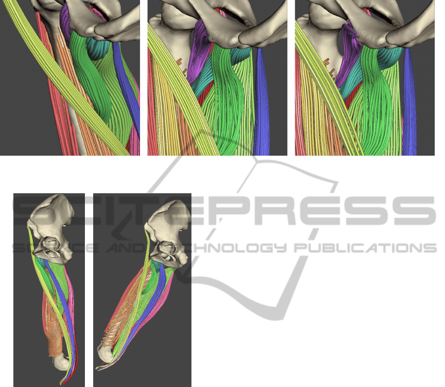
Figure 1: A detailed visualization of muscle fibres in the rest position (left), after rigid transformation to the current position

(middle) and after stabilization of the MSS (right).

Figure 2: Overview of the bone positions for the situation

depicted on Figure 1. Left is the rest position (related to

Figure 1-left) and right is the position during walking

(related to Figure 1-middle and right).

transformations are related to this position.

The first step is pre-processing, which converts

the muscle fibre polylines into particles and springs.

This is controlled by a single parameter, the number

of particles per fibre N. The fibres are divided into

N-1 uniform intervals, but instead of placing the

particles as the end points of those intervals, their

position is randomized within each interval. This is

done because when N is small and the fibres of the

muscle are roughly the same length, which is often

the case, the particles placed without randomization

tend to create clusters with large gaps in between

them and that negatively affects the CD precision

(the CD uses the particles as an approximation of the

muscle surface, therefore they should be scattered

along the surface as much as possible, details in

section 3.3).

Once the particles are created, the spring inter-

connections between them are generated using a

user-selected pattern (see 3.2 for list of implemented

patterns) and then all this is stored as simple arrays,

floating point for the particle positions and pair of

integer indices for each spring. Some other minor

structures are created during the pre-processing as

well, such as associations of particles with bones

closest to them, markings of boundary particles etc.

(see section 3.2 for details). This representation is

stored and reused through different time points un-

less the user changes some key parameters.

To process a given time point of the motion, the

transformation matrices are first applied to the

bones. The muscles (the triangular surfaces as well

as the particles) are transformed as well, using an

interpolated transformation matrix of the nearest

bones. After this basic rigid transformation, the soft-

body simulation takes place.

The simulation is an iterative process consisting

of two major parts - MSS update followed by colli-

sion handling. During the MSS update, new posi-

tions of particles are computed based on the forces

acting in the MSS. These new positions will likely

introduce some collisions with neighbouring objects

and handling those collisions in return adds some

new forces into the system. In an ideal situation,

after iterating this loop a finite number of times, the

MSS should reach an equilibrium state where no

particles move anymore. Then the final shape of the

muscles is ready and can be displayed.

However, an absolute equilibrium is obviously

practically impossible to achieve during computer

simulation. There are three possibilities of how to

end the simulation loop, each equally simple to im-

GRAPP2014-InternationalConferenceonComputerGraphicsTheoryandApplications

304

plement. In order to achieve best fidelity of the out-

put, an average displacement of the particles can be

monitored and when it falls beneath a given thresh-

old, the state is considered final. Or, if the rendering

time is more critical, a given time window, e.g.

based on the desired frame rate, can be assigned to

the computation and the output is produced immedi-

ately after this window is depleted. A compromise is

to set a fixed number of iterations.

After the final particle positions – which define

the final shape – are computed, the surface model is

updated (see 3.2) and visualized. Figures 1 and 2

show the main stages of the process on an example

of a right leg performing a common walking step.

As there are generally many time points in the

animation, the created result is discarded after the

user moves onto another time point. This unfortu-

nately slows the execution when a whole continuous

animation is wanted, as each time point is handled

separately, without exploiting the temporal coher-

ence in any way. For example, the rigid transfor-

mations from rest position to the current position

could be omitted altogether. Moreover, as it can be

expected that there will be only relatively small

changes in consecutive frames, a much smaller

number of iterations of the simulation loop would be

required to get to a plausible state in consecutive

time points. Nevertheless, the application for which

this method was designed required arbitrary time

point changes. Should the requirements change

however, the algorithm would not be difficult to

modify.

3.2 Muscle Model

There are two muscle models – the triangular sur-

face and the other is the muscle fibre model. As was

mentioned before, the key model used in the work-

load analysis is the fibre one, the surface model is

used only for the visualization. MSS are used to

represent the muscles. The MSS solver was already

implemented in the target framework, more details

about it can be found in Zelený (2011).

The solver is computing particle positions in eve-

ry time step of the simulation loop. As the particles

interconnected by springs along the muscle fibre

actually represent this fibre, it is straightforward to

obtain its new shape after the simulation ends since

it is still the same polyline, only its vertices have

different positions. However, it is not as easy to

obtain the new shape of the muscle surface. For this

reason, some relation between the particles and the

triangular model has to be established. We use mean

value coordinates (MVC) for this purpose, described

by Ju et al. (2005) as follows:

The mean value interpolation interpolates a giv-

en function f(x) defined on a closed surface by a

function g(v), v

∈R

by projecting a point p(x) of the

closed surface on a unit sphere centered at v. Then the

function value associated with p(x) is weighted by

w=[p(x)-v]

-1

and integrated over the sphere. To ensure

affine invariance, the result is divided by the weight

function integrated over the sphere S. Equation (1)

shows the result:





dSvxw

dSxfvxw

),(

)(),(

)(

(1)

The authors then continue to derive the MVC for

closed polygons and mainly triangular meshes.

Equation (2) computes the weights for point v in

regards to a given triangle with vertices p

, i = 1, 2,

3. n

are normal vectors of the three triangles vq

i-1

i+1

where q

are the vertices of a spherical triangle con-

structed by projecting the original triangle p

the unit sphere. m is the “mean vector” which is an

integral of the outward normal vector over the spher-

ical triangle surface (which is not difficult to evalu-

ate using a few trigonometric functions, see Ju et al.

(2005) for details). Weights are computed this way

for all triangles and summed analogically as in equa-

tion (1) (the integrals are replaced by sums over all

the primitives) to obtain the MVC.

)( vpn







(2)

In our case, the boundary (located on outmost fibres)

particles are triangulated and used as the source

mesh, i.e. each particle is the p(x) acting in equations

(1) and (2). Each vertex of the muscle surface mesh

is then treated as the target point (v in (1) and (2))

and its MVC are computed and stored as a pre-

processing. After the particles move during the soft-

body simulation, shape of the surface model is up-

dated simply by recalculating position of each vertex

as a linear combination of its MVC and the current

particle positions. Figure 3 shows the Gluteus max-

imus and Iliacus muscles, which change their shapes

significantly during the simulated motion – in this

case simple walking. The MVCs are used to deform

the surface from the rest pose to the final pose while

conserving the smoothness of the surface.

To simulate the tendon attachment of each mus-

cle, the particles on ends of the fibres are set as

fixed. The position of fixed particles is not updated

in the soft-body simulation, only during the rigid

transformations.

DeformableMuscleModelsforMotionSimulation

305

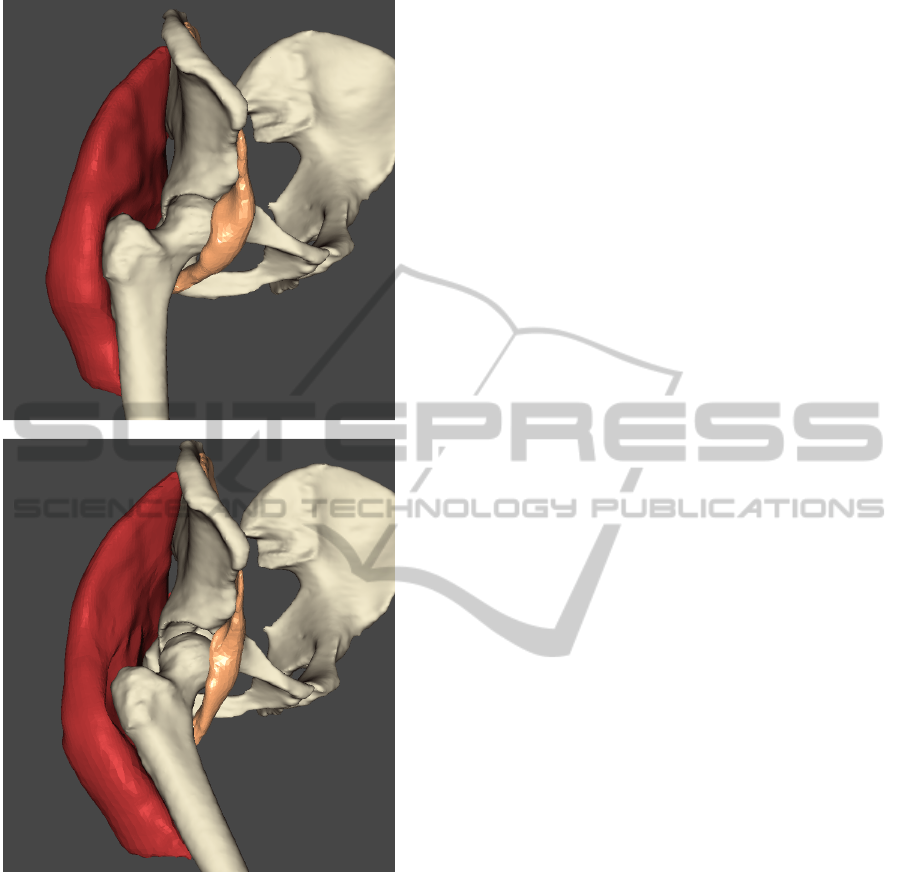
Figure 3: Surfaces of the Gluteus maximus and Iliacus

muscles. Up in rest pose (standing), down in the final pose

(walking).

There are many ways, or templates, of how to

generate the springs connecting the particles. The

more springs there are, the longer the computation

will be, but on the other hand, systems with low

spring count tend to converge to the equilibrium

state slower. Several configurations were tested:

cubic lattice with 6 or 26 springs per particle (the

particles are treated as vertices of a cubic grid with

either only the sides of the cubes being the springs,

or all sides and both face and space diagonals being

the springs); delaunay tetrahedralization (springs are

generated as edges of tetrahedrons in a delaunay

tetrahedalization of the particles); and N nearest

neighbours (each particle is connected with a user

defined number of closest particles). The impact of

the choice of the layout is discussed in Section 4.1.

3.3 Collision Handling

Collision handling is responsible for ensuring that no

objects penetrate each other. However, as section 3.2

established, the surfaces of the muscles are not in-

volved in the simulation at all. That means that one

would have to update the surface mesh in each step

of the simulation loop, detect collisions, propagate

the response onto the particles via the MVC and

continue with the simulation. This would significant-

ly increase the computation time. Another problem

is that the surfaces of individual muscles can actual-

ly intersect even in the initial position. That is not an

error in the data – some muscles can, and do, inter-

weave each other, which is easily simulated by using

the fibre model, but difficult when using the encap-

sulating surface.

To bypass these problems, the particle model it-

self is used for the collision detection (CD) instead.

Obviously, the particles represent point masses and

therefore do not have any volume. Also, they do not

necessarily trace the surface of the muscle. To

change that, the particles are thought of as spheres

with a given non-zero radius. Interpenetrations be-

tween these sets of spheres for different muscles can

then be detected and removed. At the same time

their position coincides with the particle positions

and therefore the collision response consists of noth-

ing more than updating the positions of the particles.

Another pleasing by-product of this design is simpli-

fication of the CD itself, as detecting and resolving

collisions of set of spheres is generally simpler than

in the case of triangle meshes – sphere vs. sphere

collision test is a simple comparison of their distance

and the sum of their radii. Also, only the particles

that are on the “boundary” fibres, i.e. fibres closest

to the surface, have to be accounted for – the internal

particles will not collide with other objects due to

the internal forces of the MSS.

The following heuristic has been used to obtain

the radius for each sphere. The closest particle to

each vertex of the surface mesh is found. Note that

one particle can be the closest one to several verti-

ces. To make a compromise between covering

enough of the surface of the muscle and the least of

the outside space, the radius of each sphere is set to

an average of the distances between the centre of the

particle and the associated vertices. Then the CD

mechanism is employed to detect particles that inter-

GRAPP2014-InternationalConferenceonComputerGraphicsTheoryandApplications

306

sect and their radii are decreased so that the intersec-

tion are removed, which effectively removes some

very large particles that could have been generated.

To increase the coverage of the surface without

increasing the volume excessively, more particles

per fibre can be used. However, that comes at a price

of higher memory and time demands.

For collision detection between the muscles and

bones, the same mechanism is used. The bones are

also converted to a set of spheres that approximates

their surface and then the muscle vs. bone CD is

processed in the same way as muscle vs. muscle.

The position of the spheres representing the bone

can be arbitrary (unlike in the case of muscles) and

therefore the spheres can trace the surface more

closely without taking up too much excess space.

The CD itself uses the BVH mechanism based on

the method by Larsson and Akenine-Möller (2006),

using AABBs, subdivided into even octants (i.e. the

division lines always passes through the midpoint of

the parent box). This method was chosen over the

others mentioned in Section 2.2, due to its universal-

ity and good performance documented in the afore-

mentioned work. Simple AABBs are used, because

they are faster to update as the object changes shape.

The bounding boxes are subdivided into octants in

each level of the subdivision. The division lines

always pass through the midpoint of the parent box.

Whenever new object is added to the scene, the

bounding box is constructed for it only on the parent

level, i.e. without any subdivision.

The rebuilding proposed by the original authors

(see 2.2) is not used. After testing, it has been found

out, that the proposed rules for determining whether

to rebuild part of the hierarchy does not work well in

this case. The CD is on average 5% faster when only

refitting is used. That is actually not very surprising,

as it can be expected that the shape of the muscles

will not change drastically during one simulation

step, when the particles only head toward the equi-

librium state. Also, the bounding boxes of the bones

obviously never need to be updated, because they do

not move (not in the span of one simulation step) or

change shape.

Each muscle in the scene is then tested against

each other muscle and also each bone. The BVHs of

the objects are traversed and subdivided only when

needed. The maximal number of recursion steps as

well as the minimal number of primitive per node

are either specified by a user or their default values,

empirically determined to be 8 and 10, respectively,

are used. Once either of the limits is reached, and

there is still a collision detected between the nodes, a

pair of lists containing the primitives in the two

colliding nodes is outputted and the piecewise test of

the primitives in these lists is done.

When the piecewise test detects a collision, the

difference between the distance of the two particles

and the sum of their radii is computed. Then each

particle is moved in an opposite direction to each

other by half of this distance, or eventually, if a

fixed particle is involved, the unfixed particle is

moved by the whole distance (spheres that represent

bones are treated as fixed particles). This way the

particles end up just touching each other. To take

into account that a given particle can collide with

multiple other particles, the displacement vectors are

stored and accumulated for each particle and only

after all test have been made, their superposition is

applied to the initial particle positions.

After all tests are finished, the results are applied

(i.e. the accumulated displacement vectors are used

to update the positions) and a new iteration may

begin. The particles that collided in a given time step

are treated as stopped – they are assigned a zero

velocity. This ensures that they do not rebound after

collision, which is natural for the kind of elastic

behaviour that is being simulated.

4 EXPERIMENTS

Our approach was implemented in C++ using the

VTK library (http://www.vtk.org) and integrated in a

MAF based (http://www.openmaf.org) application-

created for the VPHOP project mentioned earlier.

Figure 4: Overview of the used dataset.

DeformableMuscleModelsforMotionSimulation

307

Tests were done on a PC with Intel Core i7-3770

(3,4GHz, 4 physical cores with hyper-threading)

CPU, 8GB RAM, MS Windows 7 64-bit OS.

One data set was used for all the tests. It consists

of MRI footage of pelvis and legs, fused with a mo-

tion capture data of a walking human. A total of

twenty three muscles are available for testing in the

data set, ten of which are on the pelvis and thirteen

on the right thigh. The visualization of this dataset is

on Figure 4, with muscles rendered as surfaces.

4.1 Spring Layout

The number of iterations needed to achieve the final

shape of the soft-body affects the computational

time the most. The spring layout has a significant

impact on this number, therefore several layouts

were tested. The test processed 1500 iterations of the

simulation for each tested method, measuring the

average displacement of particles, i.e. the difference

in position of each particle between two successive

iterations. In an ideal state, the particles would not

move at all once the equilibrium position is

achieved. However, this is unlikely to happen in the

simulation. Rather than zero displacement, an oscil-

lation of the displacement values is a sign of the

final state (the positions will oscillate due to the

continuous collisions between adjacent particles).

The tested layouts were: Cubic lattice models

with 6 and 26 springs per particle, Delaunay tetrahe-

dralization (DT) and 15 nearest neighbours (see

section 3.1). The times for those methods were

111.12s, 129.6s, 124.19s and 121.37s respectively,

but please note that these times are listed only for

comparison between different spring layouts and do

not reflect the performance of the final solution – see

section 4.3 for a complete analysis of time consump-

tion. The thirteen thigh muscles were used for these

tests.

Figure 5 shows the absolute displacements for

six of the tested muscles (for better clarity of the

chart, some muscles were omitted) for the DT. The

displacement rises in the beginning as the particles

start to move faster due to the forces introduced into

the system by the initial rigid transformations. As

they reach the proximity of their final positions, their

movement slows down (after around 80 iterations),

ideally stopping entirely after more iterations.

The 26-cubic lattice and 15 nearest neighbours

have fairly similar progression as the DT on Figure

5, while the 6-cubic lattice displays almost an order

lower differences. However, note that the absolute

value of displacement measures only the differences

between consecutive iterations, not how close are

Figure 5: Absolute displacements for several muscles

simulated with the DT spring layout.

these positions to the final state. It is desirable for

the differences to actually be as high as possible.

That would mean that the model is moving fast

towards the final configuration of positions.

Figure 6 depicts the displacements for the Ad-

ductor Longus muscle (as Figure 5 documents, the

progression is quite similar for all the muscles,

therefore the choice of test subject is not important)

using four different layouts and including a linear

regression of the trend for each layout. Several first

iterations were not accounted for, because it is the

later “stabilization” phase where the differences

between individual layouts have the highest impact.

It is apparent that the 6-cubic lattice layout con-

verges at the slowest rate, while the 26-cubic is the

fastest. Even though the 6-cubic layout is the fastest

per iterations, much more iterations will be needed

in order for the model to reach the equilibrium and

therefore the execution will be the slowest. The

remaining two methods offer a reasonable compro-

mise. Various count of neighbours in the nearest

neighbour method were tested, revealing almost

strictly linear relation between the number of springs

and convergence speed.

Figure 6: Slopes of particle position displacement for the

Adductor Longus muscle.

GRAPP2014-InternationalConferenceonComputerGraphicsTheoryandApplications

308

The 6-cubic lattice is clearly the least suitable

option. Although 26-cubic lattice provides fastest

convergence, the nearest neighbour or DT layouts

also provide fast convergence while having slightly

lesser memory and computation time demands.

Moreover, if the nearest neighbour is used, the num-

ber of neighbours can be provided to the user as an

additional parameter to control the model (also note

that when using 26 neighbours, the behaviour will be

very similar to the 26-cubic). Hence, the nearest

neighbour is the suggested solution.

4.2 Deformation Quality

To compare the results of various deformation

methods, volume preservation is often used. It is

disputable whether this is a relevant metric, since the

assumption that a muscle retains its volume does not

hold in general. Nevertheless, it is one of few meas-

urable characteristics of different methods and can

reveal some relations between them. The error in

muscle volume preservation was on average 2.71%

for the used dataset. Although larger than the other,

more precise method that was available as part of the

project solution (which averaged on 0.08%), up to

6% errors are considered to be acceptable and there-

fore the presented method is usable. Moreover, by

using more fibres for the model and a larger stiffness

coefficient for the springs, the volume loss should

decrease.

More relevant evaluation method is a visual

check and comparison with real data by an expert.

Because it is almost impossible to obtain real MRI

images of the patient in different poses, medical

literature must suffice as the data in this case. The

implemented solution was handed over to a partner

facility (Istituto ortopedico Rizzoli, Italy,

http://www.ior.it) to do such evaluation test. The key

observation was that our fibre model shows “reason-

able consistency with the behaviour reported in

literature”.

The partner further investigated changes in fibre

length during motion. In general, the method per-

formed well, emulating behaviour described in med-

ical literature closely. The only complication arose

when the muscle was shortened significantly, as the

MSS-driven model tend to buckle as it was resisting

the shortening. Lower stiffness coefficients remove

this problem, but, as mentioned before, lower stiff-

ness also tend to result in higher volume error. To

conclude, in order to satisfy both the demand for low

volume error and the ability to correctly model

shortening, the stiffness coefficient must be small

and the fibre count (and therefore particle count)

high. Of course, higher particle count means slower

execution, so a balance between those parameters

has to be found. Nevertheless, the partner facility

found the method suitable for the target application.

4.3 Overall Time Performance

In order to evaluate the performance of the method,

computation times of individual steps of the simula-

tion were measured. 500 iterations of the simulation

loop were set for the test. This number was chosen

solely to obtain significant volume data for the time

measurements. In real application, less or more itera-

tions might be needed, depending on the desired

precision. Note however, that for the tested models,

500 iterations were enough to reach a state in which

the MSS start oscillating around the same values

even for the lowest particle count. Only the 13 thigh

muscles were used for this test.

Four different particle resolutions (i.e. numbers

of particles per fibre) were used for the evaluation –

20, 40, 60 and 80. While twenty particles per fibre

are sufficient to obtain acceptable output (i.e. the

model does not diverge to unnatural shapes), higher

resolution might offer better ratio between conver-

gence speed and output quality. The number of fi-

bres per muscle was always 64. While the speed of

the MSS simulation depends on the total number of

particles, the speed of CD depends only on the num-

ber of the boundary particles, as only those are in-

volved in CD. The total number of particles of the

muscles / the number of boundary particles for indi-

vidual resolution are: 1344 / 660 for resolution 20,

2624 / 1220 for 40, 3904 / 1780 for 60 and 5184 /

2340 for 80. There were three bones significant for

the used set of muscles. The same resolution (num-

ber of spheres representing the bone) was used in all

cases: 8527 spheres for the pelvis, 1568 for femur

(thigh) and 1709 for tibia (shank).

Table 1 shows the result of the test. The “MSS”

line contains the time of simulation of the MSS (the

26-cubic lattice layout was used). “Muscle CD” line

contains the time of CD of muscles vs. muscles and

the “Bones CD” contains the time of muscles vs.

bones CD. The times do not include any pre-

processing. Lastly, because the results are also af-

fected by the pose of the model (i.e. there might be

more collisions in one position than some other), the

provided times are actually an average of five differ-

ent poses of the model.

The used MSS solver is only a basic, non-

parallel implementation which can be improved on

to achieve better results. The author of the solver,

Zelený (2011), also implemented a GPU version

DeformableMuscleModelsforMotionSimulation

309

Table 1: Computation times in seconds for individual parts

of the method after 500 simulation iterations.

Resolution

Part

20 40 60 80

MSS 18.66 39.97 60.53 80.70

Muscle CD 8.15 13.50 24.00 29.53

Bones CD 30.03 37.43 56.03 67.10

TOTAL 56.84 90.9 140.56 177.33

obtaining on average 5-8x speed-up, depending on

the number of particles. However, his latest imple-

mentation cannot handle large systems due to

memory issues and would have to be modified first.

As this work was not finished yet, the CPU solver

was used here instead. Also note that the higher

computation time of CD between bones and muscles

than muscles vs. muscles is expected due to the

higher overall resolution of the bones (see above).

Table 1 shows a linear relation between the

number of particles and CD time consumption,

which is rather disappointing, as the relation should

be, in ideal case, logarithmic due to the hierarchical

structure. On average, 76% of the CD computation

time is the hierarchy traversal and 24% the piece-

wise testing. In the time counted as the piecewise

testing there is also accounted the collision response,

i.e. computing the vectors by which the spheres are

moved (see section 3.3), therefore the traversal is

considered the bottleneck.

Possible explanation of the slower-than-expected

performance is the loose fit of AABBs. As all the

objects occupy more or less the same space (they are

wrapped around the same bone), the first levels of

the hierarchy of two muscles will always intersect,

resulting in many “dead end” traversals. However,

even if for example OBBs were used instead, the

situation would not improve much as there would

still be significant overlap of the bounding volumes

due to the nature of the data.

5 CONCLUSIONS

A mass-spring model designed for representing

muscles in a musculoskeletal model was presented.

The mass-points are obtained by sampling the fibres

of the muscle. Three different ways of connecting

the particles by springs were tested. The importance

of the layout itself was found to be only marginal,

while the number of springs per particle influences

the convergence speed the most.

A collision detection and response mechanism

was designed, implemented and tested. The mecha-

nism employs bounding volume hierarchies to en-

hance the speed, the particles of the mass-spring

system are utilized as spheres of various radii ap-

proximating the surface of each object. This does not

only speed up CD tests, but also bypasses the need

to propagate changes of the shape between the sur-

face model and the mass-spring model in each itera-

tion of the simulation.

The proposed solution was evaluated by medical

experts and deemed as suitable for the purpose of

quick coarse simulations of moving human patient

and subsequent analysis of muscle deformation.

Other methods for collision detection should be

investigated further as the future work. It is the bot-

tleneck of the solution and the current mechanism

does not perform as well as expected. However, the

given task is quite complex, therefore there is no

guarantee that other algorithms will perform better.

ACKNOWLEDGEMENTS

This work has been supported by the Information

Society Technologies Programme of the European

Commission under the project VPHOP (FP7-ICT-

223865), the European Regional Development Fund

(ERDF) – project NTIS (New Technologies for

Information Society), European Centre of Excel-

lence, CZ.1.05/1.1.00/0.2.0090 and by the project

SGS-2013-029 – Advanced Computing and Infor-

mation Systems.

REFERENCES

Faure, F., Barbier, S., Allard, J., Falipou, F., 2008. Image-

based collision detection and response between arbi-

trary volume objects. In Proceedings of the 2008 ACM

SIGGRAPH/Eurographics Symposium on Computer

Animation (SCA '08). Eurographics Association, Aire-

la-Ville, Switzerland, Switzerland, 155-162.

Ju, T., Schaefer, S., Warren, J., 2005. Mean value coordi-

nates for closed triangular meshes. In ACM SIG-

GRAPH 2005 Papers (SIGGRAPH '05), Markus

Gross (Ed.). ACM, New York, NY, USA, 561-566.

Lefebvre, S., Hoppe, H., 2006. Perfect spatial hashing. In

ACM SIGGRAPH 2006 Papers (SIGGRAPH '06).

ACM, New York, NY, USA, 579-588.

Larsson, T., Akenine-Möller, T., 2006. A dynamic bound-

ing volume hierarchy for generalized collision detec-

tion. Computer Graphics 30, 3. Pergamon Press, Inc.

Elmsford, NY, USA, 450-459.

Lee, D., Glueck, M., Khan, A., Fiume, E., Jackson, K,

2012. Modeling and Simulation of Skeletal Muscle for

GRAPP2014-InternationalConferenceonComputerGraphicsTheoryandApplications

310

Computer Graphics: A Survey. Foundations and

Trends in Computer Graphics and Vision, 7, 4. Now

Publishers Inc. Hanover, MA, USA 229-276.

Lee, S.-H., Sifakis, E., Terzopoulos, D., 2009. Compre-

hensive biomechanical modeling and simulation of the

upper body. ACM Trans. Graph. 28, 4, Article 99, 17

pages.

Long, J., Burns, K., Yang, J., 2011. Cloth modeling and

simulation: a literature survey. In Proceedings of the

Third international conference on Digital human

modeling (ICDHM'11), Vincent G. Duffy (Ed.).

Springer-Verlag, Berlin, Heidelberg, 312-320.

Mendoza, C., O'Sullivan, C., 2006. Interruptible collision

detection for deformable objects. Comp. Graphics 30,

3. Pergamon Press, Inc. Elmsford, NY, USA 432-438.

Nedel, L. P., Thalmann, D., 1998. Real Time Muscle

Deformations using Mass-Spring Systems. In Pro-

ceedings of the Computer Graphics International 1998

(CGI '98). IEEE Computer Society, Washington, DC,

USA, 156-.

Tang, M., Manocha, D., Tong, R., 2009. Multi-core colli-

sion detection between deformable models. In 2009

SIAM/ACM Joint Conference on Geometric and Phys-

ical Modeling (SPM '09). ACM, New York, NY,

USA, 355-360.

Tang, Y.-M., Hui, K.-C., 2009. Simulating tendon motion

with axial mass-spring system. Comp. Graphics 33, 2.

Pergamon Press, Inc. Elmsford, NY, USA, 162-172.

Teschner, M., Heidelberger, B., Mueller, M., Pomeranets,

D., Gross, M., 2003. Optimized Spatial Hashing for

Collision Detection of Deformable Objects. In Pro-

ceedings of Vision, Modeling, Visualization VMV'03.

Munich, Germany, 47-54.

Villard, P.-F., Bourne, W., Bello, F., 2008. Modelling

Organ Deformation Using Mass-Springs and Tension-

al Integrity. In Proceedings of the 4th international

symposium on Biomedical Simulation (ISBMS '08),

Fernando Bello and P. J. Edwards (Eds.). Springer-

Verlag, Berlin, Heidelberg, 221-226.

Zelený I.: Vzájemná transformace 3D objektů reprezento-

vaných trojúhelníkovým povrchem [Morphing of 3D

objects represented by triangular surface]. Diploma

thesis, University of West Bohemia, Faculty of applied

sciences, 2011. (Available only in Czech language).

DeformableMuscleModelsforMotionSimulation

311