Discriminative Prior Bias Learning for Pattern Classification
Takumi Kobayashi and Kenji Nishida
National Institute of Advanced Industrial Science and Technology,
1-1-1 Umezono, Tsukuba, Japan
Keywords:
Pattern Classification, Discriminative Learning, Bias, SVM.
Abstract:
Prior information has been effectively exploited mainly using probabilistic models. In this paper, by focus-
ing on the bias embedded in the classifier, we propose a novel method to discriminatively learn the prior
bias based on the extra prior information assigned to the samples other than the class category, e.g., the 2-D
position where the local image feature is extracted. The proposed method is formulated in the framework of
maximum margin to adaptively optimize the biases, improving the classification performance. We also present
the computationally efficient optimization approach that makes the method even faster than the standard SVM
of the same size. The experimental results on patch labeling in the on-board camera images demonstrate the
favorable performance of the proposed method in terms of both classification accuracy and computation time.
1 INTRODUCTION
Prior information has been effectively exploited in the
fields of computer vision and machine learning, such
as for shape matching (Jiang et al., 2009), image seg-
mentation (El-Baz and Gimel’farb, 2009), graph in-
ference (Cremers and Grady, 2006), transfer learn-
ing (Jie et al., 2011) and multi-task learning (Yuan
et al., 2013). Learning prior has so far been addressed
mainly in the probabilistic framework on the assump-
tion that the prior is defined by a certain type of gener-
ative probabilistic model (Wang et al., 2010; Kapoor
et al., 2009); especially, non-parametric Bayesian ap-
proach further considers the hyper priors of the prob-
abilistic models (Ghosh and Ramamoorthi, 2003).
In this paper, we focus on the classifier, y =
w
w
w
⊤
x
x
x+b, and especially on the bias term, so called ‘b’
term (Poggio et al., 2001)
1
, while some transfer learn-
ing methods are differently built upon the prior of the
weight w
w
w for effectively transferring the knowledge
into the novel class categories (Jie et al., 2011; Gao
et al., 2012) and the prior of w
w
w also induces a regu-
larization on w
w
w. The bias is regarded as rendering the
prior information on the class probabilities (Bishop,
1995; Van Gestel et al., 2002) and we aim to learn the
1
In this paper, we describe the classifier in such a linear
form for simplicity, but our proposed method also works on
the kernel-based classifier by simply replacing the feature x
x
x
with the kernel feature φ
φ
φ
x
x
x
in the reproducing kernel Hilbert
space.
{ }
x
r
p
,
patch
,
c
c-th class label
p-th position
feature
vector
r
p=1
r
p=P
Figure 1: Patch labeling. The task is to predict the class la-
b els c of the patches, each which consists of the appearance
feature vector x
x
x and the prior position p. Note that there are
P positions in total.
unstructured prior bias b without assuming any spe-
cific models. While the bias b is generally set as a
constant across samples depending only on the class
category, in this study we define it adaptively based
on the extra prior information other than the class cat-
egory, as follows.
Suppose samples are associated with the extra
prior information p ∈ {1, ..,P} as well as the class
category c ∈ {1, ..,C}, where P and C indicate the
total number of the prior types and the class cate-
gories, respectively. For instance, in the task of la-
beling patches on the on-board camera images, each
patch (sample) is assigned with the appearance fea-
ture x
x
x, the class category c and the position (extra
prior information) p, as shown in Fig. 1. Not only
the feature x
x
x but also the prior position p where the
feature is extracted is useful to predict the class cat-
egory of the patch; the patches on an upper region
67
Kobayashi T. and Nishida K..
Discriminative Prior Bias Learning for Pattern Classification.
DOI: 10.5220/0004813600670075
In Proceedings of the 3rd International Conference on Pattern Recognition Applications and Methods (ICPRAM-2014), pages 67-75
ISBN: 978-989-758-018-5
Copyright
c
 2014 SCITEPRESS (Science and Technology Publications, Lda.)

probably belong to sky and the lower region would be
road, even though the patches extracted from those
two regions are both less textured, resulting in similar
features.
The probabilistic structure that we assume in this
study is shown in Fig. 2b with comparison to the
simple model in Fig. 2a. By using generalized linear
model (Bishop, 2006), the standard classifier (Fig. 2a)
is formulated toestimate the posterior on the class cat-
egory c as
2
logp(c|x
x
x) ∼ logp(x
x
x|c) + logp(c) = w
w
w
⊤
c
x
x
x+ b
c
, (1)
where b
c
= logp(c) indicates the class-dependent
bias. On the other hand, the
proposed model
(Fig. 2b) using the prior p induces the following clas-
sifier;
logp(c|x
x
x, p) ∼ logp(x
x
x|c) + logp(p|c) + logp(c)
= w
w
w
⊤
c
x
x
x+ b
[p]
c
, (2)
where the bias b
[p]
c
= logp(p|c) + logp(c) is depen-
dent on both the class category c and the prior infor-
mation p. Thus, if the bias could be properly deter-
mined, the classification performance would be im-
proved compared to the standard classification model
(1). One might also consider the
full-connected
model shown in Fig. 2c whose classifier is formulated
by
log p(c|x
x
x, p) ∼ log p(x
x
x|c, p) + log p(p|c) + logp(c)
= w
w
w
[p]
c
⊤
x
x
x+ b
[p]
c
, (3)
where the classifier weight w
w
w
[p]
c
relies on the prior p
as the bias b
[p]
c
does. This model is more complicated
and consumes large memory storage since the classi-
fier model {w
w
w
[p]
c
,b
[p]
c
} is prepared for respective priors
p = 1,..,P. And, due to the high degree of freedom
(D.O.F) of this model, it would be vulnerable to over-
learning. These models are summarized in Table 1
and will be again discussed later.
In this paper, we propose a novel method for
discriminatively learning the prior biases b
[p]
c
in (2)
to improve the classification performance. The pro-
posed method is formulated in the optimization prob-
lem of the maximum margin criterion (Smola et al.,
2000). We also propose the computationally efficient
approach for the optimization which contains large
amount of samples drawn from all the priors p ∈
{1,..,P}. Thereby, the proposed method is even faster
than the standard SVM (Vapnik, 1998) of the same
size, while providing the high-performance classifier
that exploits the prior information.
2
‘∼’ in (1) means the equality in disregard of the irrele-
vant constant term logp(x
x
x) or logp(x
x
x, p) in (2) and (3).
C
x
C
x
p
C
x
p
(a) simple (b) proposed (c) full-connected
Figure 2: Graphical models to depict the probabilistic de-
pendencies. The notations c, x
x
x and p denote the class cate-
gory, the (appearance) feature vector and the extra prior in-
formation, respectively. The arrows show the probabilistic
dependencies. (a) The feature x
x
x is simply drawn from the
class category c in the
simple model. (b) The proposed
model incorporates the extra prior information p which is
connected to x
x
x via c. (c) Those three variables are fully
connected in the
full-connected model.
Table 1: Classification methods for c-th class category. The
dimensionality of the feature vector is denoted by D, x
x
x ∈
ℜ
D
, and the number of prior types is P.
Method Model D.O.F
simple y
c
= w
w
w
⊤
c
x
x
x+ b
c
D+ 1
proposed y
c
= w
w
w
⊤
c
x
x
x+ b
[p]
c
D+ P
full-connected y
c
= w
w
w
[p]
c
⊤
x
x
x+ b
[p]
c
PD+ P
2 BIAS LEARNING
We detail the proposed method by first defining the
formulation for learning the biases and then present-
ing the computationallyefficient approachto optimize
them. As we proceed to describe a general form re-
garding the prior biases, it might be helpful for un-
derstanding to refer to the task of labeling patches in
on-board camera images as shown in Fig. 1; the sam-
ple is represented by the appearance feature x
x
x and the
prior position p ∈ {1, ..,P}.
2.1 Formulation
We consider a binary class problem for simplicity and
take a one-vs-rest approach for multi-class tasks. Sup-
pose we have P types of prior information, and let
x
x
x
[p]
i
∈ ℜ
D
denote the D-dimensional feature vector of
the i-th sample (i = 1,..,n
[p]
) drawn from the p-th type
of prior. As described in Sec.1, we deal with the clas-
sification defined by
y = w
w
w
⊤
x
x
x
[p]
+ b
[p]
, (4)
where y denotes the classifier output which is sub-
sequently thresholded by zero for performing binary
classification, and w
w
w and b
[p]
are the classifier weight
vector and the bias, respectively. Note again that
ICPRAM2014-InternationalConferenceonPatternRecognitionApplicationsandMethods
68

the bias b
[p]
depends on the p-th type of prior, p ∈
{1,..,P}. The classifier (4) can be learned via the fol-
lowing optimization formulation in the framework of
maximum margin (Smola et al., 2000);
min
w
w
w,{b
[p]
}
p
1
2
kw
w
wk
2
+C
P
∑
p
n
[p]
∑
i
ξ
[p]
i
(5)
s.t. ∀p ∈ {1, .., P}, ∀i ∈ {1,..,n
[p]
},
y
[p]
i
(w
w
w
⊤
x
x
x
[p]
i
+ b
[p]
) ≥ 1 − ξ
[p]
i
, ξ
[p]
i
≥ 0,
where C is the cost parameter. This is obviously con-
vex and its Lagrangian is written by
L =
1
2
kw
w
wk
2
+C
P
∑
p
n
[p]
∑
i
ξ
[p]
i
−
P
∑
p
n
[p]
∑
i
β
[p]
i
ξ
[p]
i
(6)
−
P
∑
p
n
[p]
∑
i
α
[p]
i
{y
[p]
i
(w
w
w
⊤
x
x
x
[p]
i
+ b
[p]
) − 1+ ξ
[p]
i
},
where we introduce the Lagrange multipliers α
[p]
i
≥
0, β
[p]
i
≥ 0. The derivatives of the Lagrangian are
∂L
∂w
w
w
= w
w
w−
P
∑
p
n
[p]
∑
i
α
[p]
i
y
[p]
i
x
x
x
[p]
i
= 0
0
0
⇒ w
w
w =
P
∑
p
n
[p]
∑
i
α
[p]
i
y
[p]
i
x
x
x
[p]
i
(7)
∂L
∂ξ
[p]
i
= C− α
[p]
i
− β
[p]
i
= 0 ⇒ 0 ≤ α
[p]
i
≤ C (8)
∂L
∂b
[p]
=
n
[p]
∑
i
α
[p]
i
y
[p]
i
= 0. (9)
Thereby, the dual is finally obtained as
min
{α
[p]
i
}
i,p
1
2
P
∑
p,q
n
[p]
∑
i
n
[q]
∑
j
α
[p]
i
α
[q]
j
y
[p]
i
y
[q]
j
x
x
x
[p]
i
⊤
x
x
x
[q]
j
−
P
∑
p
n
[p]
∑
i
α
[p]
i
(10)
s.t. ∀p,
n
[p]
∑
i
α
[p]
i
y
[p]
i
= 0, ∀i,∀p, 0 ≤ α
[p]
i
≤ C.
This is a quadratic programming (QP) analogous to
the dual of SVM (Vapnik, 1998) except that there ex-
ist P linear equality constraints with respect to α
α
α
[p]
.
The standard QP solver is applicable to optimize
(10), though requiring substantial computation cost.
For optimizing QP of the SVM dual, the method of
SMO (Platt, 1999) is successfully applied, but in this
case, we can not employ it directly due to the multiple
equality constraints. In what follows, we present the
computationally efficient approach to optimize (10).
2.2 Optimization
A large number of variables {α
[p]
i
}
i,p
in the QP (10)
are inherently partitioned into block-wise variables
regarding the prior p; we obtain P blocks of α
α
α
[p]
=
{α
[p]
i
}
i=1,..,n
[p]
∈ ℜ
n
[p]
, p = 1,..,P. According to those
block-wise variables, (10) is decomposed into the fol-
lowing sub-problem as well:
min
α
α
α
[p]
i
1
2
n
[p]
∑
i, j
α
[p]
i
α
[p]
j
y
[p]
i
y
[p]
j
x
x
x
[p]
i
⊤
x
x
x
[p]
j
−
n
[p]
∑
i
α
[p]
i
(
1− y
[p]
i
P
∑
q6=p
n
[q]
∑
j
α
[q]
j
y
[q]
j
x
x
x
[p]
i
⊤
x
x
x
[q]
j
)
(11)
s.t.
n
[p]
∑
i
α
[p]
i
y
[p]
i
= 0, ∀i, 0 ≤ α
[p]
i
≤ C.
This is again a quadratic programming which resem-
bles the SVM dual except for the linear term with re-
spect to α
α
α
[p]
and thus is effectively optimized by using
the SMO (Platt, 1999). Therefore, the whole proce-
dure for optimizing (10) consists of iteratively opti-
mizing the sub-problem (11) with respect to the prior
p by means of SMO as shown in Algorithm 1.
In order to discuss the convergence of the itera-
tive optimization, we mention the KKT condition of
(10) (Fan et al., 2005). The optimizer α
[p]
i
satisfies the
following condition:
G
i,p
(α
α
α) + b
[p]
i
y
[p]
i
= λ
[p]
i
− µ
[p]
i
, (12)
λ
[p]
i
α
[p]
i
= 0, µ
[p]
i
(C − α
[p]
i
) = 0, λ
[p]
i
≥ 0, µ
[p]
i
≥ 0,
where G
i,p
(α
α
α) = y
[p]
i
x
x
x
[p]
i
⊤
∑
P
q
∑
n
[q]
j
α
[q]
j
y
[q]
j
x
x
x
[q]
j
−1 is the
derivative of the objective function in (10) with re-
spect to α
[p]
i
. This is rewritten into
α
[p]
i
< C : G
i,p
(α
α
α) + b
[p]
i
y
[p]
i
≥ 0, (13)
α
[p]
i
> 0 : G
i,p
(α
α
α) + b
[p]
i
y
[p]
i
≤ 0, (14)
and since y
[p]
i
∈ {+1,−1}, the aboveconditions result
in
−y
[p]
i
G
i,p
(α
α
α)
(
≤ b
[p]
i
i ∈ I
[p]
+
≥ b
[p]
i
i ∈ I
[p]
−
, (15)
where
I
[p]
+
={i|(α
[p]
i
<C∧ y
[p]
i
=1) ∨ (α
[p]
i
>0∧ y
[p]
i
=−1)},
(16)
I
[p]
−
={i|(α
[p]
i
<C∧ y
[p]
i
=−1) ∨ (α
[p]
i
>0∧ y
[p]
i
=1)}.
(17)
DiscriminativePriorBiasLearningforPatternClassification
69

Therefore, we can conclude that α
[p]
i
is a stationary
point if and only if
δ
[p]
,

max
i∈I
[p]
+
−y
[p]
i
G
i,p
(α
α
α)

−

min
i∈I
[p]
−
−y
[p]
i
G
i,p
(α
α
α)

≤ 0.
(18)
On the basis of this measure, we can stop the it-
eration when max
p
δ
[p]
< ε with a small tolerance
ε > 0. The measure δ
[p]
also provides a clue for
effectively selecting the prior p to be optimized via
(11). That is, we perform the (sub-)optimization (11)
at p
∗
= argmax
p
δ
[p]
so as to effectively minimize
max
p
δ
[p]
. This approach will be empirically validated
in the experiment. At the optimum, the bias b
[p]
is re-
trieved by
b
[p]
=
1
|I
[p]
|
∑
i∈I
[p]
−y
[p]
i
G
i,p
(α
α
α), (19)
where I
[p]
= {i|0 < α
[p]
i
< C}, (20)
since the right hand side in (12) equals zero for i ∈ I
[p]
.
Finally, we describe the technical tip for further
reducing the computational cost in the optimization.
From a practical viewpoint, the samples of the two
class categories are not equally distributed across the
priors p = 1, .., P but are localized in limited number
of priors. For instance, in the case of on-board cam-
era images, the road never appears in upper regions
where the sky usually dominates. That is, we occa-
sionally encounter the following sub-problem;
min
α
α
α
[p]
i
1
2
n
[p]
∑
i, j
α
[p]
i
α
[p]
j
y
[p]
i
y
[p]
j
x
x
x
[p]
i
⊤
x
x
x
[p]
j
−
n
[p]
∑
i
α
[p]
i
(
1− y
[p]
i
P
∑
q6=p
n
[q]
∑
j
α
[q]
j
y
[q]
j
x
x
x
[p]
i
⊤
x
x
x
[q]
j
)
(21)
s.t.
n
[p]
∑
i
α
[p]
i
y
[p]
i
= 0, ∀i, 0 ≤ α
[p]
i
≤ C, (22)
∀i, y
[p]
i
= 1
(or ∀i, y
[p]
i
= −1). (23)
The above QP is trivially optimized by α
α
α
[p]
= 0
0
0 due to
the constraint (22), and the bias b
[p]
can be determined
as
b
[p]
=
(
+∞ ∀i, y
[p]
i
= 1
−∞ ∀i, y
[p]
i
= −1
, (24)
which means that the samples from such a prior are
definitely classified as positive (or negative) no matter
how the appearance features of the samples are. In
this case, the class category is solely dependent on the
prior information via the bias b
[p]
∈ {+∞,−∞}. This
setting (24) might be too excessive and more mild one
Algorithm 1: Bias Learning.
Input: {x
x
x
[p]
i
,y
[p]
i
}: feature vector and its class label
of the i-th training sample from the p-th type of
prior, p = 1,..,P, i = 1,..,n
[p]
.
ε > 0: small tolerance for terminating the it-
eration.
1: P = {p|∃i, y
[p]
i
= 1∧ ∃i,y
[p]
i
= −1}
2: Initialization: ∀p ∈ {1,..,P}, α
α
α
[p]
= 0
0
0
3: Randomly pick up p ∈ P
4: repeat
5: Set α
α
α
[p]
as the optimizer of (11)
6: Compute δ
[p]
in (18), ∀p ∈ P
7: p ← argmax
p∈P
δ
[p]
8: until max
p∈P
δ
[p]
< ε
Output: w
w
w computed by (7) and {b
[p]
}
p=1,..,P
com-
puted by (19) for p ∈ P and (24) for p /∈ P, using
the optimizers {α
α
α
[p]
}
p
.
would be preferable for the classification; this is our
future work. By eliminating such trivial types of prior,
we can reduce the computational burden of the whole
procedure to optimize (10). As a result, the proposed
optimization procedure is shown in Algorithm 1.
2.3 Discussion
In the proposed method, all samples across all types
of priors are leveraged to train the classifier, improv-
ing the generalization performance. In contrast, the
full-connected method (Table 1) treats the samples
separately regarding the priors, and thus the p-th clas-
sifier is learnt by using only a small amount of sam-
ples belonging to the p-th type of prior, which might
degrade the performance. On the other hand, the
simple method learning the classifier from the whole
set of samples is less discriminative without utiliz-
ing the prior information associated with the samples.
The proposed method effectivelyintroduces the priors
into the classifiers via the biases which are discrimi-
natively optimized.
The proposed method is slightly close to the cross-
modal learning (Kan et al., 2012; Sharma and Jacobs,
2011). The samples belonging to different priors are
separated as if they are in different modalities, though
the feature representations are the same in this case.
The proposed method deals with them in a unified
manner via the adaptive prior biases. Actually, the
proposed method is applicable to the samples that are
distributed differently across the priors; the sample
distribution is shifted (translated) as x
x
x
[q]
= x
x
x
[p]
+e
e
e and
the prior bias can adapt to it by b
[q]
= b
[p]
−w
w
w
⊤
e
e
e since
y
[p]
= w
w
w
⊤
x
x
x
[p]
+ b
[p]
, y
[q]
= w
w
w
⊤
x
x
x
[q]
+ b
[q]
= w
w
w
⊤
x
x
x
[p]
+
ICPRAM2014-InternationalConferenceonPatternRecognitionApplicationsandMethods
70

On-board image Label image
Figure 3: CamVid dataset (Brostow et al., 2008).
(b
[q]
+ w
w
w
⊤
e
e
e) = y
[p]
. Therefore, the samples of the dif-
ferent priors are effectively transferred into the opti-
mization to improve the classification performance.
3 EXPERIMENTAL RESULTS
We evaluated the proposed method on patch label-
ing in the on-board camera images by using CamVid
dataset (Brostow et al., 2008). This patch labeling
contributes to understand the scene surrounding the
car.
3.1 Setting
The CamVid dataset (Brostow et al., 2008) contains
several sequences composed of fully labeled image
frames as shown in Fig. 3: each pixel is assigned with
one of 32 class labels including ‘void’. Those labeled
images are captured at 10 Hz. In this experiment, we
employ the major 11 labels frequently seen in the im-
age frames, road, building, sky, tree, sidewalk, car,
column pole, sign symbol, fence, pedestrian and bicy-
clist, to form the 11-class classification task.
We extracted the GLAC image feature (Kobayashi
and Otsu, 2008) from a local image patch of 20 × 40
pixels which slides at every 10 pixels over the resized
image of 480 × 360. In this case, the feature vector
x
x
x ∈ ℜ
2112
is associated with the 2D position of the
patch as the extra prior information; the total number
of prior types (grid points) is P = 1551. Thus, the task
is to categorize the patch feature vectors extracted at
1511 positions into the above-mentioned 11 classes.
We used the three sequences in the CamVid
dataset, and partitioned each sequence into three sub-
sequences along the time, one of which was used for
training and the others were for test. This cross vali-
dation was repeated three times and the averaged clas-
sification accuracy is reported.
For comparison, we applied the methods men-
tioned in Sec.1;
simple and full-connected meth-
ods as listed in Table 1. The simple method is a stan-
dard classification using the weight w
w
w with the bias
b without relying on the prior information p. The
full-connected method applies classifiers compris-
ing w
w
w
[p]
and b
[p]
at respective priors p = 1,..,P.
This method requires tremendous memory storage
for those P classifiers; in this experiment, 2112-
dimensional weight vectors w
w
w in 11 class categories
are stored at each of 1511 positions. On the other
hand, in the
proposed method, the feature vectors
are classified by using the identical weight w
w
w across
the priors together with the adaptively optimized bias
b
[p]
depending on the prior p.
3.2 Computation Cost
We evaluated the proposed method in terms of com-
putation cost.
The first issue is related to the way of selecting
p in the iterative optimization; the proposed proce-
dure selects p deterministically by p
∗
= argmax
p
δ
[p]
(the 7-th line in Algorithm 1). As the alternative for
the proposed selection, the other two ways are con-
ceivable, sequential and random selections. In the se-
quential selection, the target prior p is simply selected
as in raster scan over the image frame. The random
selection means that the target p is randomly picked
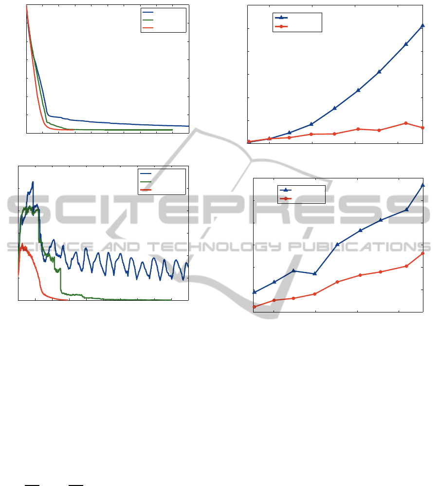
up from the whole set {1,..,P}. Fig. 4 shows the com-
parison results with respect to the objective cost in
(10) and the gap max
p
δ
[p]
in (18) measuring viola-
tion of the KKT condition, both of which should be
decreased toward convergence. The optimization is
fast converged via the proposed method, while in the
other methods the optimization takes a larger num-
ber of iterations until convergence; in particular, the
sequential method requires more than 10,000 itera-
tions. These results reveal the importance of selecting
p to be optimized and show that the proposed method
quickly decreases the cost as well as the gap, leading
to fast convergence.
The second issue is about scalability of the pro-
posed method. The method trains the classifier by us-
ing all the samples across the priors, scale of which
is as large as in the
simple method. Fig. 5a shows
the computation time with comparison to the
simple
method on various sizes of training samples. These
methods are implemented by MATLAB using lib-
svm (Chang and Lin, 2001) on Xeon 3.33GHz PC
3
.
The proposed method is significantly faster than the
simple method. The time complexity of simple
method which solves the standard SVM dual has been
empirically shown to be O(n
2.1
) (Joachims, 1999).
The proposedoptimization approachiteratively works
3
In this experiment, the feature vectors are actually con-
verted into the form of the kernel Gram matrix to which the
QP solver in libsvm is directly applied, for fair comparison
of the QP problems in the
proposed and simple methods.
DiscriminativePriorBiasLearningforPatternClassification
71

500 1000 1500 2000 2500 3000 3500 4000 4500 5000
−1400
−1200
−1000
−800
−600
−400
−200
0
Cost
Iterations
sequential
random
proposed
(a) Objective cost
500 1000 1500 2000 2500 3000 3500 4000 4500 5000
0
2
4
6
8
10
12
Gap
Iterations
sequential
random
proposed
(b) Gap, max
p
δ
[p]
Figure 4: Comparison for the ways of selecting the target
prior p in terms of (a) the objective cost in (10) and (b)
the gap max
p
δ
[p]
in (18) which measures violation of KKT
condition.
on the block-wise subset into which the whole train-
ing set is decomposed (Sec.2.2). The subset is re-
garded as the working set whose size is an important
factor for fast computing QP (Fan et al., 2005). In the
proposed method, it is advantageous to inherently
define the subset, i.e., the working set, of adequate
size according to the prior. Thus, roughly speaking,
the time complexity of the
proposed method results
in O(M
n
2.1
M
2.1
) = O(
n
2.1
M
1.1
). In particular, the computa-
tion time essentially depends on the (resultant) num-
ber of support vectors (SVs); Fig. 5b shows the num-
ber of support vectors produced by those two meth-
ods. The
proposed method provides a smaller num-
ber of support vectors, which significantly contributes
to reduce the computation time. As a result, the
proposed optimization approach works quite well to-
gether with the working set (prior p) selection dis-
cussed in the previous experiment (Fig. 4). These re-
sults show the favorable scalability of the
proposed
method, especially compared to the standard simple
5000 10000 20000 30000 40000
0
10
20
30
40
50
60
Number of training samples
Computation time (sec)
simple
proposed
(a) Computation time
5000 10000 20000 30000 40000
0
1000
2000
3000
4000
5000
6000
Number of training samples
Number of SVs
simple
proposed
(b) Number of support vectors (SVs)
Figure 5: Comparison of the
simple and proopsed meth-
ods in terms of (a) computation time as well as (b) number
of support vectors (SVs).
method.
3.3 Classification Performance
We then compared the classification performance of
the three methods,
simple , full-connected and
proposed (Table 1). Table 2 shows the overall per-
formance, demonstrating that the
proposed method
outperforms the others. It should be noted that
the
full-connected method individually applies the
classifier specific to the prior p ∈ {1,,P}, requiring
a plenty of memory storage and consequently taking
large classification time due to loading the enormous
memory. The
proposed method renders as fast clas-
sification as the simple method since it enlarges only
the bias. By discriminativelyoptimizing the biases for
respective priors, the performance is significantly im-
proved in comparison to the
simple method; the im-
provement is especially found at the categories of car,
pedestrian and bicyclist that are composed of patch
ICPRAM2014-InternationalConferenceonPatternRecognitionApplicationsandMethods
72

−inf
−9
−8
−7
−6
−5
−4
+inf
−inf
−5.5
−5
−4.5
−4
−3.5
−3
−2.5
−2
−1.5
+inf
−inf
−1
−0.5
0
0.5
1
1.5
2
2.5
3
3.5
+inf
road building sky
−inf
−5
−4.5
−4
−3.5
−3
−2.5
−2
−1.5
−1
+inf
−inf
−3
−2.5
−2
−1.5
−1
−0.5
0
0.5
+inf
−inf
−14
−13.5
−13
−12.5
−12
−11.5
−11
−10.5
−10
−9.5
−9
+inf
tree sidewalk car
−inf
−5.5
−5
−4.5
−4
−3.5
−3
+inf
−inf
−9
−8.5
−8
−7.5
+inf
−inf
−2.6
−2.4
−2.2
−2
−1.8
−1.6
−1.4
+inf
column pole sign symbol fence
−inf
−1
−0.5
0
0.5
1
+inf
−inf
−6.5
−6
−5.5
−5
+inf
pedestrian bicyclist
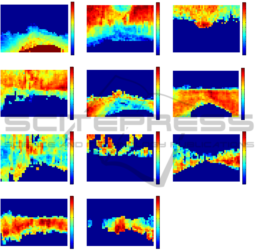
Figure 6: Maps of the biases learnt by the proposed method. The significance of the biases are shown by using pseudo colors
from (dark) blue to (dark) red. This figure is best viewed in color.
parts similar to other categories but are associated
with the distinct prior positions.
Finally, we show in Fig. 6 the biases learnt by
the
proposed method; the biases {b
[p]
}
p
are folded
into the form of image frame according to the x-y po-
sitions. These maps of the biases reflect the prior
probability over the locations where the target cat-
egory appears. These seem quite reasonable from
the viewpoint of the traffic rules that the car obeys;
since the CamVid dataset is collected at the Cam-
bridge city (Brostow et al., 2008), in this case, the
traffic rules are of the United Kingdom. The high
biases for the sky are distributed above the horizon-
tal line, while those of the road are high in the lower
part. The pedestrian probably walks on the sidewalk
mainly shown in the left side. The oncoming car runs
on the right-hand road, and the row of the building
is found on the roadside. These biases are adaptively
learnt from the CamVid dataset and they would be dif-
ferent if we use other datasets collected under differ-
ent traffic rules.
DiscriminativePriorBiasLearningforPatternClassification
73

Table 2: Classification accuracy (%).
simple full-connected proposed
road 93.10 93.80 94.92
building 75.90 72.96 78.70
sky 90.52 82.21 90.25
tree 70.49 77.59 79.95
sidewalk 77.06 78.43 81.36
car 53.84 58.64 65.16
column pole 9.53 16.15 12.85
sign symbol 1.73 1.62 1.70
fence 5.23 11.09 13.48
pedestrian 17.26 30.69 31.52
bicyclist 17.09 18.49 24.88
avg. 46.52 49.24 52.25
4 CONCLUSIONS
We have proposed a method to discriminatively learn
the prior biases in the classification. In the proposed
method, for improving the classification performance,
all samples are utilized to train the classifier and the
input sample is adequately classified based on the
prior information via the learnt biases. The proposed
method is formulated in the maximum-margin frame-
work, resulting in the optimization problem of the QP
form similarly to SVM. We also presented the compu-
tationally efficient approach to optimize the resultant
QP along the line of SMO. The experimental results
on the patch labeling in the on-board camera images
demonstrated that the proposed method is superior in
terms of classification accuracy and the computation
cost. In particular, the proposed classifier operates
as fast as the standard (linear) classifier, and besides
the computation time for training the classifier is even
faster than the SVM of the same size.
REFERENCES
Bishop, C. M. (1995). Neural Networks for Pattern Recog-
nition. Oxford University Press, New York, NY.
Bishop, C. M. (2006). Pattern Recognition and Machine
Learning. Springer, Berlin, Germany.
Brostow, G. J., Shotton, J., Fauqueur, J., and Cipolla, R.
(2008). Segmentation and recognition using structure
from motion point clouds. In ECCV’08, the 10th Eu-
ropean Conference on Computer Vision, pages 44–57.
Chang, C.-C. and Lin, C.-J. (2001). LIBSVM: a library
for support vector machines. Software available at
http://www.csie.ntu.edu.tw/ cjlin/libsvm.
Cremers, D. and Grady, L. (2006). Statistical priors for ef-
ficient combinatorial optimization via graph cuts. In
ECCV’06, the 9th European Conference on Computer
Vision, pages 263–274.
El-Baz, A. and Gimel’farb, G. (2009). Robust image seg-
mentation using learned priors. In ICCV’09, the 12nd
International Conference on Computer Vision, pages
857–864.
Fan, R.-E., Chen, P.-H., and Lin, C.-J. (2005). Working set
selection using second order information for training
support vector machines. Journal of Machine Learn-
ing Research, 6:1889–1918.
Gao, T., Stark, M., and Koller, D. (2012). What makes a
good detector? - structured priors for learning from
few examples. In ECCV’12, the 12th International
Conference on Computer Vision, pages 354–367.
Ghosh, J. and Ramamoorthi, R. (2003). Bayesian Nonpara-
metrics. Springer, Berlin, Germany.
Jiang, T., Jurie, F., and Schmid, C. (2009). Learning shape
prior models for object matching. In CVPR’09, the
22nd IEEE Conference on Computer Vision and Pat-
tern Recognition, pages 848–855.
Jie, L., Tommasi, T., and Caputo, B. (2011). Multi-
class transfer learning from unconstrained priors. In
ICCV’11, the 13th International Conference on Com-
puter Vision, pages 1863–1870.
Joachims, T. (1999). Making large-scale svm learning prac-
tical. In Sch¨olkopf, B., Burges, C., and Smola, A.,
editors, Advances in Kernel Methods - Support Vec-
tor Learning, pages 169–184. MIT Press, Cambridge,
MA, USA.
Kan, M., Shan, S., Zhang, H., Lao, S., and Chen, X. (2012).
Multi-view discriminant analysis. In ECCV’12, the
12th International Conference on Computer Vision,
pages 808–821.
Kapoor, A., Hua, G., Akbarzadeh, A., and Baker, S. (2009).
Which faces to tag: Adding prior constraints into ac-
tive learning. In ICCV’09, the 12nd International
Conference on Computer Vision, pages 1058–1065.
Kobayashi, T. and Otsu, N. (2008). Image feature extraction
using gradient local auto-correlations. In ECCV’08,
the 10th European Conference on Computer Vision,
pages 346–358.
Platt, J. (1999). Fast training of support vector machines
using sequential minimal optimization. In Sch¨olkopf,
B., Burges, C., and Smola, A., editors, Advances
in Kernel Methods - Support Vector Learning, pages
185–208. MIT Press, Cambridge, MA, USA.
Poggio, T., Mukherjee, S., Rifkin, R., Rakhlin, A., and
Verri, A. (2001). b. Technical Report CBCL Paper
#198/AI Memo #2001-011, Massachusetts Institute of
Technology, Cambridge, MA, USA.
Sharma, A. and Jacobs, D. (2011). Bypassing synthesis:
Pls for face recognition with pose, low-resolution and
sketch. In CVPR’11, the 24th IEEE Conference on
Computer Vision and Pattern Recognition (CVPR),
pages 593–600.
Smola, A. J., Bartlett, P., Sch¨olkopf, B., and Schuurmans,
D. (2000). Advances in Large-Margin Classifiers.
MIT Press, Cambridge, MA, USA.
ICPRAM2014-InternationalConferenceonPatternRecognitionApplicationsandMethods
74

Van Gestel, T., Suykens, J., Lanckriet, G., Lambrechts, A.,
De Moor, B., and Vandewalle, J. (2002). Bayesian
framework for least squares support vector machine
classifiers, gaussian processes and kernel fisher dis-
criminant analysis. Neural Computation, 15(5):1115–
1148.
Vapnik, V. (1998). Statistical Learning Theory. Wiley, New
York, NY, USA.
Wang, C., Liao, X., Carin, L., and Dunson, D. (2010). Clas-
sification with incomplete data using dirichlet process
priors. The Journal of Machine Learning Research,
11:3269–3311.
Yuan, C., Hu, W., Tian, G., Yang, S., and Wang, H. (2013).
Multi-task sparse learning with beta process prior for
action recognition. In CVPR’13, the 26th IEEE Con-
ference on Computer Vision and Pattern Recognition,
pages 423–430.
DiscriminativePriorBiasLearningforPatternClassification
75