On the Use of Copulas in Joint Chance-constrained Programming
Michal Houda and Abdel Lisser
Laboratoire de Recherche en Informatique, Universit
´
e Paris Sud – XI, B
ˆ
at. 650, 91405 Orsay Cedex, France
Keywords:
Chance-constrained Programming, Dependence, Archimedean Copulas, Second-Order Cone Programming.
Abstract:
In this paper, we investigate the problem of linear joint probabilistic constraints with normally distributed
constraints. We assume that the rows of the constraint matrix are dependent, the dependence is driven by
a convenient Archimedean copula. We describe main properties of the problem and show how dependence
modeled through copulas translates to the model formulation. We also develop an approximation scheme for
this class of stochastic programming problems based on second-order cone programming.
1 INTRODUCTION
Consider an uncertain linear optimization problem
minc
T
x subject to Ξx ≤h, x ∈ X (1)
where x ∈X ⊂R
n
is a decision vector of the problem,
Ξ ∈ R
K
×R
n
is an uncertain (unknown) data matrix,
c ∈ R
n
, h = (h
1
,...,h
K
)
T
∈ R
K
are fixed determin-
istic vectors, dimensions n, K are structural elements
of the optimization problem (1). If a realization of the
data element Ξ is known and fixed in advance (before
a decision is taken), we can solve the problem (1) as
classical linear optimization problem. This situation
is rarely the case. More often, we have to consider
uncertainty of the data as natural element of the mod-
eling phase.
During the history of mathematical optimization,
various methods were developed to deal with the un-
certainty: ex-post sensitivity analysis, parametric pro-
gramming, or robust optimization. In our paper, we
concentrate on the stochastic programming approach
assuming that the data matrix Ξ is a random matrix
whose probabilistic characteristics are known in ad-
vance. For example, if the constraints of (1) are re-
quired to be satisfied with a prescribed sufficiently
high probability p ∈ [0; 1], then the problem (1) can
be reformulated as
minc
T
x subject to P{Ξx ≤h} ≥ p, x ∈ X (2)
where p ∈[0; 1] is a prescribed probability level. The
problem (2) is known as probabilistically (or chance)
constrained linear optimization problem. The prob-
lem was treated many times in literature; for a thor-
ough review of methods and bibliography we refer to
the classical book (Pr
´
ekopa, 1995) and recent chap-
ters (Pr
´
ekopa, 2003) and (Dentcheva, 2009).
The chance constrained optimization problems are
very challenging in their general (linear or nonlinear)
form. Two main issues of the stochastic optimization
theory concerning these problems are the convexity of
the set of feasible solutions, and a very high compu-
tational effort to be accomplished. In detail: even for
the “nice” linear program (2) the feasible set may be
nonconvex, and the probability P can result in an in-
tractable computation of multivariate integrals.
In our paper, we restrict our consideration to a
problem with linear normally distributed constraint
rows, namely, the rows Ξ
T
k
of Ξ follow n-dimensional
normal distributions with means µ
k
and positive def-
inite covariance matrices Σ
k
. To further simplify the
situation we assume that X = R
n
(only the probabilis-
tic constraints are in question). Denote
X(p) :=

x ∈R
n
| P{Ξx ≤ h} ≥ p

. (3)
We are interested in an equivalent formulation of
the set X (p) convenient for numerical purposes. To
this end, we first present a result for the set
M(p) :=

x ∈R
n
|P
{
g
k
(x) ≥ ξ
k
, k = 1,...,K
}
≥ p

,
(4)
where ξ := (ξ
1
,...,ξ
K
) is an absolutely continuous
random vector and g
k
(x) are continuous functions.
M(p) is usually referred to as the set of feasible so-
lutions for a continuous chance-constrained problem
with random right-hand side.
The convexity of the sets X(p) and M(p) is treated
several times in the literature; we mention (Miller and
Wagner, 1965), (Pr
´
ekopa, 1971), (Jagannathan, 1974)
as the first classical results, and (Henrion, 2007),
72
Houda M. and Lisser A..
On the Use of Copulas in Joint Chance-constrained Programming.
DOI: 10.5220/0004831500720079
In Proceedings of the 3rd International Conference on Operations Research and Enterprise Systems (ICORES-2014), pages 72-79
ISBN: 978-989-758-017-8
Copyright
c
 2014 SCITEPRESS (Science and Technology Publications, Lda.)

(Henrion and Strugarek, 2008), (Pr
´
ekopa et al., 2011)
as recently published papers. These results are sim-
plified either by restricting consideration to one-row
problem only, or by assuming independence of ma-
trix rows. In our paper we demonstrate the use of
copula theory to deal with dependence of rows in (2).
This was done first by (Henrion and Strugarek, 2011)
for the set M(p) using a class of so-called logexp-
concave copulas. We extend their results to another
large, more usual class of copulas and formulate an
equivalent description of the problem (2) convenient
to be solved by methods of second-order cone pro-
gramming.
2 DEPENDENCE
2.1 Basic Facts about Copulas
Theory of copulas is well known for the people of
probability theory and mathematical statistics but, to
our knowledge, was not used up to these days in
stochastic programming to describe the structure of
the problem. In this section, we mention only some
basic facts about copulas necessary for our following
investigation. Most of the notions here (up to Propo-
sition 2.7) were taken from the book (Nelsen, 2006).
Definition 2.1. A copula is the distribution function
C : [0; 1]
K
→ [0;1] of some K-dimensional random
vector whose marginals are uniformly distributed on
[0;1].
Proposition 2.2 (Sklar’s Theorem). For any K-
dimensional distribution function F : R
K
→ [0; 1]
with marginals F
1
,...,F
K
, there exists a copula C
such that
∀z ∈ R
K
F(z) = C(F
1
(z
1
),.. . , F
K
(z
K
)). (5)
If, moreover, F
k
are continuous, then C is uniquely
given by
C(u) = F(F
−1
1
(u
1
),.. . , F
−1
K
(u
K
)). (6)
Otherwise, C is uniquely determined on range F
1
×
···×rangeF
K
.
Through Sklar’s Theorem, we have in hand an ef-
ficient general tool for handling an arbitrary depen-
dence structure. First, if we know the marginal dis-
tributions F
k
together with the copula representing
the dependence we can unambiguously determine the
joint distribution. On the other hand, the copula can
be uniquely derived from the knowledge of the joint
and all marginal distributions. Our first example is the
independent (product) copula which is nothing else
than the independence formula for distribution func-
tions:
C
Π
(u) =
∏
k
u
k
. (7)
The second important example is the Gaussian cop-
ula which is given by Sklar’s Theorem applied to a
joint normal distribution and its normally distributed
marginals:
C
Σ
(u) = Φ
Σ
(Φ
−1
(u
1
),.. . , Φ
−1
(u
K
)) (8)
where Φ
Σ
is the distribution function of the multivari-
ate normal distribution with zero mean, unit variance
and covariance matrix Σ, and Φ
−1
(u
k
) are standard
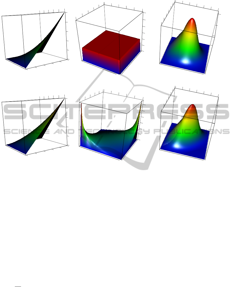
one-dimensional normal quantiles. For illustration
purposes, we provide a set of figures (Figures 1–5)
of some popular copulas. From the left-hand side, the
reader can always find the distribution function of the
copula (i. e., the copula itself), its density, and the den-
sity of the distribution given by the copula applied to
the standard normal marginals. Figure 1 represents
the independent copula; compare it to the Gaussian
copula in Figure 2. Note that the Gaussian copula
is the only copula that can represent the joint normal
distribution.
The following proposition provides the limits in
which the copulas can be located.
Proposition 2.3 (The Fr
´
echet-Hoeffding bounds).
Every copula C satisfies the inequalities
W (u) ≤C(u) ≤C
M
(u) (9)
where
W (u) := max

∑
u
k
−K + 1, 0

,
C
M
(u) := min
k
{u
k
}.
The function W represents the completely nega-
tive dependence between marginal distributions, but
it is known not to be a copula if K > 2. C
M
represents
the completely positive dependence and it is known
under the name of the comonotone (maximum) cop-
ula. These functions together with the independent
copula are often found to be limiting cases of some
other classes of copulas.
The Gaussian copula has a rather complicated
structure (even it is not analytic) to be treated directly
in our optimization problems. Instead, we need a dif-
ferent, simpler class of copulas, which we found in
so-called Archimedean copulas.
Definition 2.4. A copula C is called Archimedean if
there exists a continuous strictly decreasing function
ψ : [0; 1] → [0;+∞], called generator of C, such that
ψ(1) = 0 and
C(u) = ψ
−1
n
∑
i=1
ψ(u
i
)
!
. (10)
OntheUseofCopulasinJointChance-constrainedProgramming
73

x
0
y
0.2
0.4
0.6
0.8
1
0
0.2
0.4
0.6
0.8
z
0
0.2
0.4
0.6
0.8
1
1
x
1
0
0.5
1
1.5
0
0.2
0.4
0.6
0.8
1
2
2.5
3
y
0.2
0.4
0.6
0.8
z
0
x
y
-1
-2
-3
3
2
1
z
-3
-2
-1
0
0
1
0
2
0.05
0.1
3
0.15
Figure 1: Independent copula: distribution, density, and density with standard normal marginals.
x
0
z
0
0.2
0.4
0.6
0.8
1
y
0.2
0.4
0.6
0.8
1
0
0.2
0.4
0.6
0.8
1
x
1
0
1
2
0
0.2
0.4
0.6
0.8
1
3
4
5
6
y
0.8
0.2
0.4
0.6
z
0
x
y
-2
3
-3
2
1
0
z
0
0
1
-1
0.05
2
0.1
3
0.15
-3
-2
-1
Figure 2: Gaussian copula (ρ = 0.55): distribution, density, and density with standard normal marginals.
If lim
t→0
ψ(t) = +∞ then C is called a strict
Archimedean copula and ψ is called a strict gener-
ator.
The inverse ψ
−1
of a generator function is contin-
uous and strictly decreasing on [0; ψ(0)] (the value of
ψ(0) is defined as +∞ if the copula is strict). Some-
times, ψ
−1
is defined as the generalized inverse on the
whole positive half-line [0; +∞) by setting ψ
−1
(s) =
0 for s ≥ ψ(0) but such a definition is not needed
through the context of our paper. To determine if
some continuous strictly decreasing function ψ is a
copula generator we introduce the following notion.
Definition 2.5. A real function f : R → R is called
completely monotonic on an open interval I ⊆ R if it
is nondecreasing, differentiable for each order k, and
its derivatives alternate in sign, i. e.
(−1)
k
d
k
dt
k
f (t) ≥ 0 ∀k = 0,1,..., and ∀t ∈I. (11)
Proposition 2.6. Let ψ : [0; 1] → R
+
be a strictly de-
creasing function with ψ(1) = 0 and lim
t→0
ψ(t) =
+∞. Then it is a generator of a strict Archimedean
copula for each dimension K ≥2 if and only if ψ
−1
is
completely monotonic on (0;+∞).
The extension of Proposition 2.6 given by (McNeil
and Ne
ˇ
slehov
´
a, 2009) has the following corollary:
Proposition 2.7. Any copula generator is convex.
The Archimedean copulas are considered as a fa-
vorable and useful class of copulas due to their pos-
sibly simple formulation by a simple analytic func-
tion ψ and a small number of parameters (usually one
or two). Many families adapted to concrete problem
settings were already given in the literature; for ex-
ample, the book (Nelsen, 2006) provides a table of
22 one-parameter families of Archimedean copulas.
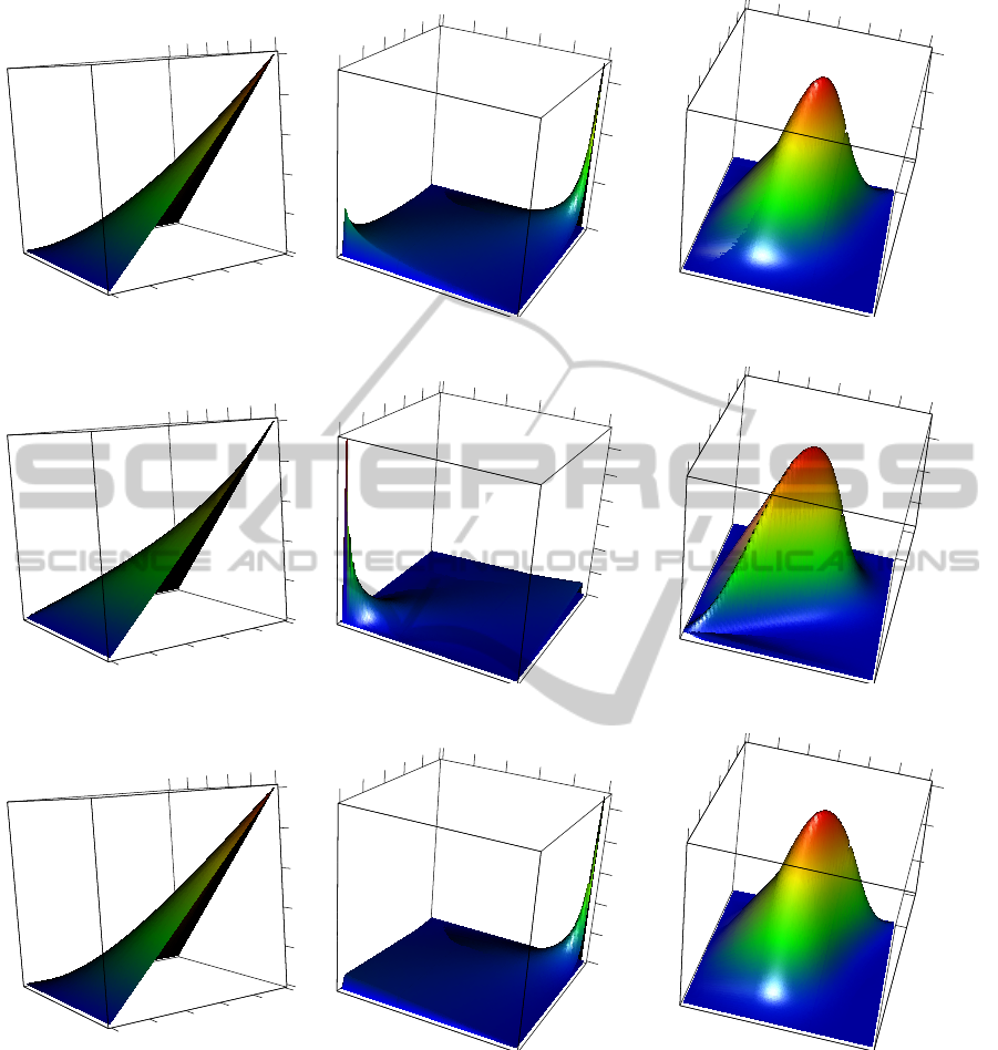
We give some examples in Table 1 and Figures 3–
5. The Gumbel-Hougaard and Joe copulas are asym-
metric (in the sense of density contours for normal
marginals) stressing the dependence of positive ran-
dom variables; the Clayton copula is in a similar view
useful to model the positive dependence of negative
random variables. The Frank copulas have symmetric
density contours for normal marginals.
The Archimedean copulas provide an easy equiv-
alent formulation for feasible sets (3) and (4). We
start with the set M(p); assume (for each k = 1, . . . , K)
that the elements ξ
k
of ξ have continuous distribution
functions F
k
, and the whole vector ξ has the joint dis-
tribution induced by a copula C. With these assump-
ICORES2014-InternationalConferenceonOperationsResearchandEnterpriseSystems
74

x
0
y
0.2
0.4
0.6
0.8
1
0
0.2
0.8
0.6
0.4
1
z
0
0.2
0.4
0.6
0.8
1
x
1
0
0.2
0.4
0.6
0.8
0
5
10
15
1
0.8
0.6
y
0.4
0.2
z
0
x
y
0
z
1
0.05
0
-1
2
0.1
0.15
3
0.2
-2
3
-3
2
1
-3
-2
-1
0
Figure 3: Gumbel-Hougaard copula (θ = 1.6): distribution, density, and density with standard normal marginals.
x
0
y
z
0
0.2
0.4
0.6
0.8
1
0.2
0.4
0.6
0.8
1
0
0.2
0.4
0.6
0.8
1
x
1
0
5
10
0
0.2
0.4
0.6
0.8
1
15
20
25
30
0.8
y
0.6
0.4
0.2
z
0
x
y
0
0.05
3
-3
-2
1
2
z
0
-1
1
2
0.1
3
0.15
0.2
-3
-2
-1
0
Figure 4: Clayton copula (θ = 1.8): distribution, density, and density with standard normal marginals.
x
0
z
0
0.2
0.4
0.6
0.8
1
y
0.2
0.4
0.6
0.8
1
0
0.2
0.4
0.6
0.8
1
x
1
5
0
0.2
0.4
0.6
0.8
1
10
15
20
25
0.6
0.8
0.4
0.2
0
y
0
z
x
y
0
z
1
2
0
0.05
-1
0.1
3
0.15
-2
0.2
3
-3
2
-3
-2
-1
0
1
Figure 5: Joe copula (θ = 2.1): distribution, density, and density with standard normal marginals.
tions, we can rewrite the set M(p) as
M(p) =

x |C

F
1
(g
1
(x),..., F
K
(g
K
(x))

≥ p

(12)
and prove the following lemma.
Lemma 2.8. If the copula C is Archimedean with a
(strict or non-strict) generator ψ then
M(p) =

x | ∃y
k
≥ 0 :
ψ[F
k
(g
k
(x))] ≤ ψ(p)y
k
∀k,
K
∑
k=1
y
k
= 1

. (13)
Proof. From basic properties of ψ it is easily seen that
M(p) =

x | ψ
−1

K
∑
k=1
ψ[F
k
(g
k
(x))]

≥ p

=

x ∈R
n
|
K
∑
k=1
ψ[F
k
(g
k
(x))] ≤ ψ(p)

.
(14)
Assume that there exists nonnegative variables y =
(y
1
,... , y
K
) with
∑
k
y
k
= 1 such that (13) holds. Then
the inequality in (14) can be easily obtained by sum-
OntheUseofCopulasinJointChance-constrainedProgramming
75

Table 1: Selected Archimedean copulas with completely
monotonic inverse generators.
Copula family Param. θ Gen. ψ
θ
(t)
Independent (product) – −lnt
Gumbel-Hougaard θ ≥1 (−lnt)
θ
Clayton θ > 0
1
θ
(t
−θ
−1)
Joe θ ≥1 −ln[1 −(1 −t)
θ
]
Frank θ > 0 −ln

e
−θt
−1
e
−θ
−1

ming up all the inequalities in (13). The existence of
such vector y for the case p = 1 is obvious; hence as-
sume p < 1 and define
y
k
:=
ψ

F
k
(g
k
(x))

ψ(p)
for k = 1,...,K −1,
y
K
:= 1 −
K−1
∑
k=1
y
k
.
It is now easy to verify that such definition of y
k
sat-
isfies (13).
2.2 Introducing Normal Distribution
Return our consideration to the set X(p) of the linear
chance constrained problem defined by (3). Assume
that the constraint rows Ξ
T
k
have n-variate normal dis-
tributions with means µ
k
and covariance matrices Σ
k
.
For x 6= 0 define
ξ
k
(x) :=
Ξ
T
k
x −µ
T
k
x
p
x
T
Σ
k
x
, g
k
(x) :=
h
k
−µ
T
k
x
p
x
T
Σ
k
x
. (15)
The random variable ξ
k
(x) has one-dimensional stan-
dard normal distribution (in particular, this distribu-
tion is independent of x). Therefore the feasible set
can be written as
X(p) =
n
x | P

ξ
k
(x) ≤ g
k
(x) ∀k

≥ p
o
. (16)
If K = 1 (i. e., there is only one row constraint), the
feasible set can be simply rewritten as
X(p) =
n
x | µ
T
1
x + Φ
−1
(p)
p
x
T
Σ
1
x ≤h
1
o
. (17)
where, again, Φ
−1
is the one-dimensional standard
normal quantile function. Introducing auxiliary vari-
ables y
k
and applying Lemma 2.8, we derive the fol-
lowing lemma which gives us an equivalent descrip-
tion of the set X(p) using the copula notion.
Lemma 2.9. Suppose, in (3), that Ξ
T
k
∼ N(µ
k
,Σ
k
)
(with appropriate dimensions) where Σ
k
 0. Then
the feasible set of the problem (2) can be equivalently
written as
X(p) =
n
x | ∃y
k
≥ 0 :
∑
k
y
k
= 1,
µ
k
T
x + Φ
−1

ψ
−1
(y
k
ψ(p))

p
x
T
Σ
k
x ≤h
k
∀k
o
(18)
where Φ is the distribution function of a standard
normal distribution and ψ is the generator of an
Archimedean copula describing the dependence prop-
erties of the rows of the matrix Ξ.
Proof. Straightforward using the arguments given
above. The remaining case x = 0 is obvious.
2.3 Convexity
It is not easy to show the convexity of the sets M(p)
and X(p). We drop this question out of this paper and
refer to (Houda and Lisser, 2013) where the convexity
of both sets was proven under the conditions that
1. p is sufficiently high, and
2. ψ
−1
is completely monotonic.
The proof was based on the theory presented in (Hen-
rion and Strugarek, 2008) for the case of indepen-
dence, and (Henrion and Strugarek, 2011) for the case
of dependence modeled via logexp-concave copulas.
Our approach is different and makes direct use of the
convexity property of Archimedean generators. See
the references above for details.
3 MAIN RESULT
3.1 Convex Reformulation
In Lemma 2.9 we have already stated an equivalent
formulation of the feasible set X(p). Together with
the previous notice on convexity we can formulate the
following theorem.
Theorem 3.1. Consider the problem (2) where
1. the matrix Ξ has normally distributed rows Ξ
T
k
with means µ
k
and positive definite covariance
matrices Σ
k
;
2. the joint distribution function of ξ
k
(x) given by
(15) is driven by an Archimedean copula with the
generator ψ.
Then the problem (2) can be equivalently written as
minc
T
x subject to
µ
k
T
x + Φ
−1

ψ
−1
(y
k
ψ(p))

p
x
T
Σ
k
x ≤h
k
,
∑
k
y
k
= 1
x ∈X, y
k
≥ 0 with k = 1,...,K.
(19)
ICORES2014-InternationalConferenceonOperationsResearchandEnterpriseSystems
76

Moreover, if
3. the function ψ
−1
is completely monotonic;
4. p > p
∗
:= Φ

max{
√
3,4λ
(k)
max
[λ
(k)
min
]
−3/2
kµ
k
k}

,
where λ
(k)
max
,λ
(k)
min
are the largest and lowest eigen-
values of the matrices Σ
k
, and Φ is the one-
dimensional standard normal distribution func-
tion,
then the problem is convex.
The value of the minimal probability level p
∗
was
given by (Henrion and Strugarek, 2008) and it does
not change for our dependent case.
3.2 SOCP Approximation
Second-order cone programming (SOCP) is a sub-
class of convex optimization in which the problem
constraint set is the intersection of an affine linear
manifold and the Cartesian product of second-order
(Lorentz) cones (Alizadeh and Goldfarb, 2003). For-
mally, a constraint of the form
kAx + bk
2
≤ e
T
x + f
is a second-order cone constraint as the affine func-
tion (Ax + b,e
T
x + f ) is required to lie in the second-
order cone {(y,t) | kyk
2
≤ t}. The linear and con-
vex quadratic constraints are nominal examples of
second-order cone constraints. It is easy to see that
the constraint (17) is SOCP constraint with A := Σ
1
,
b := 0, e := −
1
Φ
−1
(p)
µ
1
, and f :=
1
Φ
−1
(p)
h
1
provided
p ≥
1
2
. For a details about SOCP methodology we re-
fer the reader to (Alizadeh and Goldfarb, 2003), and
to the monograph (Boyd and Vandenberghe, 2004).
Theorem 3.1 provides us an equivalent nonlinear
convex reformulation of the linear chance-constrained
problem (2). Due to the decision variables y
k
ap-
pearing as arguments to the (nonlinear) quantile func-
tion Φ
−1
, it is not still a second-order cone formu-
lation. To resolve this computational issue, we for-
mulate a lower and upper approximation to the prob-
lem (19) using the favorable convexity property of the
Archimedean generator. We first formulate an auxil-
iary convexity lemma which gives us a possibility to
find these approximations.
Lemma 3.2. If p > p
∗
(given in Theorem 3.1), and
ψ is a generator of an Archimedean copula, then the
function
y 7→ H(y) := Φ
−1

ψ
−1
(yψ(p))

(20)
is convex on [0;1].
Proof. The function ψ
−1
(·) is a strictly decreasing
convex function on [0; ψ(0)] with values in [p;1]; the
function Φ
−1
(·) is non-decreasing convex on (p
∗
;1].
Hence, the function H(y) is convex.
The proposed approximation technique follows
the outline appearing in (Cheng and Lisser, 2012) and
(Cheng et al., 2012). For both the approximations that
follow, we consider a partition of the interval (0;1] in
the form 0 < y
k1
< ... < y
kJ
≤ 1 (for each variable
y
k
).
Remark 3.3. The number J of partition points can dif-
fer for each row index k but, to simplify the notation
and without loss of generality, we consider this num-
ber to be the same for each index k.
3.2.1 Lower Bound: Piecewise Tangent
Approximation
We approximate the function H(y
k
) using the first
order Taylor approximation at each of the partition
points; the calculated Taylor coefficients a
k j
, b
k j
translate into the formulation of the problem (19) as
the linear and SOCP constraints with additional aux-
iliary nonnegative variables z
k
and w
k
. The convexity
of H(·) ensures that the resulting optimal solution is a
lower bound for the original problem.
Theorem 3.4. Given the partition points y
k j
, con-
sider the problem
minc
T
x subject to
µ
k
T
x +
p
z
kT
Σ
k
z
k
≤ h
k
,
z
k
≥ a
k j
x + b
k j
w
k
(∀k, ∀j)
∑
k
w
k
= x,
w
k
≥ 0, z
k
≥ 0 (∀k),
(21)
where
a
k j
:= H(y
k j
) −b
k j
y
k j
,
b
k j
:=
ψ(p)
φ(H(y
k j
))ψ
0

ψ
−1
(y
k j
ψ(p))

,
and φ be the standard normal density. Then the op-
timal value of the problem (21) is a lower bound for
the optimal value of the problem (2).
Remark 3.5. The linear functions a
k j
+ b
k j
y are tan-
gent to the (quantile) function H
k
at the partition
points; hence the origin of the name tangent approx-
imation. This approximation leads to an outer bound
for feasible solution set X(p).
OntheUseofCopulasinJointChance-constrainedProgramming
77

3.2.2 Upper Bound: Piecewise Linear
Approximation
The line passing through the two successive partition
points with their corresponding values H(y
k j
) is an
upper linear approximation of H(y
k
) between these
two successive points. Taking pointwise maximum of
these linear functions we arrive to an upper approxi-
mation of the function H, hence to an upper bound for
the optimal value of the original problem.
Theorem 3.6. Given partition points y
k j
, consider
the problem
minc
T
x subject to
µ
k
T
x +
p
z
kT
Σ
k
z
k
≤ h
k
,
z
k
≥ a
k j
x + b
k j
w
k
(∀k, j < J)
∑
k
w
k
= x,
w
k
≥ 0, z
k
≥ 0 (∀k)
(22)
where
a
k j
:= H(y
k j
) −b
k j
y
k j
,
b
k j
:=
H(y
k, j+1
) −H(y
k j
)
y
k, j+1
−y
k j
.
Then the optimal value of the problem (22) is an upper
bound for the optimal value of the problem (2).
The last two problems are second-order cone pro-
gramming problems and they are solvable by standard
algorithms of SOCP. We do not provide further details
in our paper; some promising numerical experiments
were done by (Cheng and Lisser, 2012) for the prob-
lem with independent rows. If the dependence level
is not too high (for example, if the parameter θ of the
Gumbel-Hougaard copula approaches to one) the re-
sulting approximation bounds are comparable to this
independent case.
The second-order cone programming approach
to solve chance-constrained programming problems
opens a great variety of ways how to solve real-life
problems. Many applications are modeled through
chance-constrained programming: among them we
can choose for example
• applications from finance: asset liability man-
agement, portfolio selection (covering necessary
payments through an investment period with high
probability),
• engineering applications in energy and other in-
dustrial areas (dealing with uncertainties in energy
markets and/or weather conditions),
• water management (designing reservoir systems
with uncertain stream inflows),
• applications in supply chain management, pro-
duction planning, etc.
We refer the reader to the book (Wallace and Ziemba,
2005) for a diversified set of applications from these
(and other) areas and for ideas how uncertainty is in-
corporated into the models by the stochastic program-
ming approach. The method proposed in this paper
shifts the research and open new possibilities as the
constraint dependence is in fact a natural property of
constraints involved in all mentioned domains.
4 CONCLUSIONS
In our paper, we have presented a way how copulas
can be used to translate a known result for chance-
constrained optimization problems with independent
constraint rows to the case where the constraints ex-
hibit some dependence. More specifically: if we as-
sume that the dependence can be represented by a
strict Archimedean copula with the completely mono-
tonic generator inverse, the convexity of the feasible
set is assured for sufficiently high values of p, and
an equivalent deterministic formulation can be given.
Furthermore, a lower and an upper bound for the op-
timal value of the problem can be calculated by intro-
ducing the piecewise tangent and piecewise linear ap-
proximations of the quantile function and by solving
the associated second-order cone programming prob-
lems.
ACKNOWLEDGEMENTS
This work was supported by the Fondation
Math
´
ematiques Jacques Hadamard, PGMO/IROE
grant No. 2012-042H.
REFERENCES
Alizadeh, F. and Goldfarb, D. G. (2003). Second-order cone
programming. Mathematical Programming, 95(1):3–
51.
Boyd, S. P. and Vandenberghe, L. (2004). Convex Optimiza-
tion. Cambridge University Press. Seventh printing
with corrections, 2009.
Cheng, J., Gicquel, C., and Lisser, A. (2012). A second-
order cone programming approximation to joint
chance-constrained linear programs. In Mahjoub,
A., Markakis, V., Milis, I., and Paschos, V., editors,
Combinatorial Optimization, volume 7422 of Lecture
ICORES2014-InternationalConferenceonOperationsResearchandEnterpriseSystems
78

Notes in Computer Science, pages 71–80. Springer
Berlin / Heidelberg.
Cheng, J. and Lisser, A. (2012). A second-order cone
programming approach for linear programs with joint
probabilistic constraints. Operations Research Let-
ters, 40(5):325–328.
Dentcheva, D. (2009). Optimization models with proba-
bilistic constraints. In Shapiro, A., Dentcheva, D., and
Ruszczy
´
nski, A., editors, Lectures on Stochastic Pro-
gramming: Modeling and Theory, volume 9 of MOS-
SIAM Series on Optimization, pages 87–153. SIAM,
Philadelphia.
Henrion, R. (2007). Structural properties of linear proba-
bilistic constraints. Optimization, 56(4):425–440.
Henrion, R. and Strugarek, C. (2008). Convexity of chance
constraints with independent random variables. Com-
putational Optimization and Applications, 41(2):263–
276.
Henrion, R. and Strugarek, C. (2011). Convexity of chance
constraints with dependent random variables: The use
of copulae. In Bertocchi, M., Consigli, G., and Demp-
ster, M. A. H., editors, Stochastic Optimization Meth-
ods in Finance and Energy, volume 163 of Interna-
tional Series in Operations Research & Management
Science, pages 427–439. Springer, New York.
Houda, M. and Lisser, A. (2013). Second-order cone pro-
gramming approach for elliptically distributed joint
probabilistic constraints with dependent rows. Re-
search Report 1566, Laboratoire de Recherche en In-
formatique, Universit
´
e Paris Sud XI.
Jagannathan, R. (1974). Chance-constrained program-
ming with joint constraints. Operations Research,
22(2):358–372.
McNeil, A. J. and Ne
ˇ
slehov
´
a, J. (2009). Multivariate
Archimedean copulas, d-monotone functions and `
1
-
norm symmetric distributions. Annals of Statistics,
37(5B):3059–3097.
Miller, B. L. and Wagner, H. M. (1965). Chance constrained
programming with joint constraints. Operations Re-
search, 13(6):930–945.
Nelsen, R. B. (2006). An Introduction to Copulas. Springer,
New York, 2nd edition.
Pr
´
ekopa, A. (1971). Logarithmic concave measures with
applications to stochastic programming. Acta Scien-
tiarium Mathematicarum (Szeged), 32:301–316.
Pr
´
ekopa, A. (1995). Stochastic Programming. Akad
´
emiai
Kiad
´
o, Budapest.
Pr
´
ekopa, A. (2003). Probabilistic programming. In
Ruszczy
´
nski, A. and Shapiro, A., editors, Stochastic
Programming, volume 10 of Handbooks in Opera-
tions Research and Management Science, pages 267–
352. Elsevier, Amsterdam.
Pr
´
ekopa, A., Yoda, K., and Subasi, M. M. (2011). Uniform
quasi-concavity in probabilistic constrained stochas-
tic programming. Operations Research Letters,
39(3):188–192.
Wallace, S. W. and Ziemba, W. T., editors (2005). Applica-
tions of Stochastic Programming, volume 5 of MPS-
SIAM Series on Optimization. SIAM, Philadelphia.
OntheUseofCopulasinJointChance-constrainedProgramming
79