
Image Decolorization by Maximally Preserving Color Contrast
Alex Yong-Sang Chia
1
, Keita Yaegashi
2
and Soh Masuko
2
1
Institute for Infocomm Research, Singapore, Singapore
2
Rakuten Inc., Shinagawa-ku, Tokyo, Japan
Keywords:
Image Decolorization, Feature Representation.
Abstract:
We propose a method to convert a color image to its gray representation with the objective that color contrast
in the color image is maximally preserved as gray contrast in the gray image. Given a color image, we first
extract unique colors of the image through robust clustering for its color values. Based on the color contrast
between these unique colors, we tailor a non-linear decolorization function that maximally preserves contrast
in the gray image. A novelty here is the proposal of a color-gray feature that tightly couple color contrast with
gray contrast information. We compute the optimal color-gray feature, and drive the search for a decolorization
function that generates a color-gray feature that is most similar to the optimal one. This function is then used
to convert a color image to its gray representation. Our experiments and user study demonstrate the greater
effectiveness of this method in comparison to previous techniques.
1 INTRODUCTION
Image decolorization refers to the process of convert-
ing a color image to its gray representation. This con-
version is important in applications such as gray scale
printing, single channel image/video processing, and
image rendering for display on monochromatic de-
vices e.g. ebook readers. This is a dimension reduc-
tion problem, which inevitably results in information
loss in the gray image. Correspondingly, the goal in
image decolorization is to ensure as much appearance
of a color image is retained in the gray image as pos-
sible. In this work, we aim to generate a gray image
such that color contrast that is visible in a color im-
age is maximally retained as gray contrast in the gray
image. This ensures different colored patches (both
connected and disjoint) of the color image can be dis-
tinguished as different gray patches in the gray im-
age. Given that a color image can have arbitrary col-
ors that are randomly distributed across the image, de-
colorization with the focus that contrast preservation
is maximized is a hard image processing problem.
A key contribution in this paper is the proposal of
a novel color-gray feature which tightly couples color
contrast of a color image with the gray contrast infor-
mation of its gray image. This representation affords
us with several unique advantages. First, by encap-
sulating both color and gray contrast information into
a single representation, it allows us to directly eval-
uate the quality of a gray image based on informa-
tion available in its color image. More importantly,
it empowers us with a convenient avenue to define an
optimal feature that represents the maximum preser-
vation of color contrast in the form of gray contrast
in the gray image. Consequently, by searching for
a color-gray feature that is most similar to the opti-
mal feature, we can compute a gray image in which
different colored regions in the color image are also
distinguishable in the gray image.
We employ a non-linear decolorization function
to convert a color image to a gray image. The use
of a non-linear function increases the search space
for the optimal gray image. To reduce computation
cost, we adopt a coarse-to-fine search strategy which
quickly eliminates unsuitable parameters of the decol-
orization function to hone in on the optimal parameter
values. We show through experimental comparisons
that the proposed decolorization method outperforms
the state-of-the-art methods.
This paper is organized as follows. Immediately
below, we discuss related works. We present our de-
colorization method in Sect. 2. Experimental evalua-
tions against existing methods are detailed in Sect. 3.
Finally, we conclude in Sect. 4.
1.1 Related Work
Traditional decolorization methods apply a weighted
sum to each of the color planes to compute a gray
453
Yong-Sang Chia A., Yaegashi K. and Masuko S..
Image Decolorization by Maximally Preserving Color Contrast.
DOI: 10.5220/0004862104530459
In Proceedings of the 3rd International Conference on Pattern Recognition Applications and Methods (ICPRAM-2014), pages 453-459
ISBN: 978-989-758-018-5
Copyright
c
2014 SCITEPRESS (Science and Technology Publications, Lda.)

value for each pixel. For example, Matlab (MAT-
LAB, 2010) eliminates the hue and saturation com-
ponents from a color pixel, and retain the luminance
component as the gray value for each pixel. (Neu-
mann et al., 2007) conducted a large scale user study
to identify the general set of parameters which per-
form best on most images, and used these parameters
to design their decolorization function. Such meth-
ods support very fast computation for the gray val-
ues, in which the computational complexity is O(1).
However, given that the decolorization function is not
tailored to the input image, decolorization results of
these methods often provide does not maintain maxi-
mal information presented in the color image.
Modern approaches to convert a color image to
its gray representation tailor a decolorization function
to the color image. Such approaches can be clas-
sified into two main categories, local mapping and
global mappings. In local mapping approaches, the
decolorization function applies different color-to-gray
mappings to image pixels based on their spatial posi-
tions. For example, (Bala and Eschbach, 2004) en-
hanced color edges by adding high frequency com-
ponents of chromaticity to the luminance component
of a gray image. (Smith et al., 2008) used a local
mapping step to map color values to gray values, and
utilized a local sharpening step to further enhance the
gray image. While such methods to enhance the lo-
cal features can improve the perceptually quality of
the gray representation, a weakness of these methods
is that they could distort the appearance of uniform
color regions. This may results in haloing artifacts.
Global mapping methods use a decolorization
function that applies the same color-to-gray mapping
to all image pixels. (Rasche et al., 2005) proposed an
objective function which combines the needs to main-
tain contrast of an image with consistency of the lumi-
nance channel. A constrained multi-variate optimiza-
tion framework is used to find the gray image which
optimizes the objective function. (Gooch et al., 2005)
constrained their optimization on neighboring pixel
pairs, where they sought to preserve color contrast be-
tween pairs of image pixels. (Kim et al., 2009) devel-
oped a fast decolorization method which seeks to pre-
serve image feature discriminability and reasonable
color ordering. Their method is based on the obser-
vation that more saturated colors are perceived to be
brighter than their luminance values. Recently, (Lu
et al., 2012) proposed a method which first defines a
bimodal objective function, and then uses a discrete
optimization framework to find a gray image which
preserves color contrast. As one weakness, (Gooch
et al., 2005; Kim et al., 2009; Lu et al., 2012) op-
timize contrast between neighboring connected pixel
pairs and does not consider color/gray differences be-
tween non-connected pixels. Hence, different col-
ored regions that are non-connected may be mapped
to similar gray values by their methods. This results
in the loss of appearance information in the gray im-
age. Our framework considers both connected and
non-connected pixel pairs to find the optimal decol-
orization function of an image and thus does not suf-
fer from this shortcoming.
2 OUR APPROACH
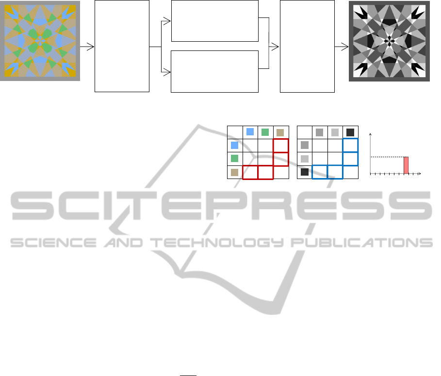
Fig. 1 outlines our method which comprises four
main modules. Given a color image, we first extract
unique colors from the image. We compute the cor-
responding gray values of these color values using a
currently considered decolorization function. Based
on these color and gray values, we compute a color-
gray feature to encapsulate the color and gray contrast
information into a single representation. The best
possible color-gray feature is computed and we eval-
uated the quality of the currently considered decol-
orization function by comparing its color-gray feature
with the optimal one. Here, a coarse-to-fine search
strategy is employed to search for a decolorization
function which provides the color-gray feature that is
a closest fit to the optimal feature. In this aspect, our
method explicitly drives the search towards the gray
image which maximally preserves the color contrast
in the form of gray contrast. This function is then
used to convert the color image into its gray represen-
tation. We elaborate on these modules next.
2.1 Extracting Unique Colors
Given an input color image, we first extract its unique
color values by applying the robust mean shift clus-
tering method of (Cheng, 1995) on its color values.
Let
{
c
i
}
denote the set of clusters formed. We do not
remove weakly populated clusters, but instead con-
sider all mean shift clusters for subsequent process-
ing. Consequently, the color clusters represent not
only dominant colors of the image, but collectively
represent the unique colors of the image.
We highlight three advantages of using these
unique colors in the decolorization framework. First,
it affords our method with lower computational cost
as compared to methods which operate on a per-pixel
basis, since the number of unique colors is typically
much less than the number of image pixels. Second,
as the clusters represent all unique colors that are ex-
tracted from the image, therefore it does not concen-
trate the color-to-gray optimization on only the dom-
ICPRAM2014-InternationalConferenceonPatternRecognitionApplicationsandMethods
454
Coarse-to-
fine search
Section 2.4
Input color image
Resulting gray image
Extracting
unique
colors
Section 2.1
Extracting
color
-
gray
features
Section 2.2
Deriving
optimal
color-gray feature
Section 2.3
Figure 1: System overview of our decolorization method.
inant color space of the image (but instead on the en-
tire color space represented by the image). Most im-
portantly, these color clusters do not include spatial
information of pixels. Consequently, by focusing the
search for an optimal decolorization function across
these color clusters, it empowers our method to op-
timize on a global image basis rather than on a local
neighborhood basis. This ensures different colored
regions which are non-connected to map to gray re-
gions that are distinguishable.
2.2 Extracting Color-gray Features
We first discuss the non-linear decolorization func-
tion that we adopt to convert a color image to its gray
counterpart, before describing the computation for a
color-gray feature.
Given a pixel p of a color image, we define its red,
green and blue components as
{
p
r
, p
g
, p
b
}
in which
the values varies within the range of 0 to 1. Let p
gray
denote the gray value of pixel p. We compute p
gray
by the multivariate non-linear function,
p
gray
= ((p
r
)
x
× w
r
+ (p
g
)
y
× w
g
+ (p
b
)
z
× w
b
)
3
x+y+z
,
(1)
where
{
w
r
, w
g
, w
b
}
are weight values and
{
x, y, z
}
are
the power values that correspond to the red, green
and blue components respectively. The non-linear
function increases the search space (and affords much
flexibility) to find an optimal gray representation. Our
aim here is to find the best set of weight and power
values that results in maximal retention of color con-
trast in the form of gray contrast in the image.
We now describe the computation of a color-gray
feature which tightly couples color contrast to gray
contrast. For each cluster c
i
obtained in Sect. 2.1,
we first compute its mean color value from all pix-
els within the cluster. We compute the Euclidean dis-
tance between the mean color values of all clusters,
and collect the color distances into a distance ma-
trix Φ. Additionally, for each cluster, we compute
the gray values for all pixels within the cluster based
on a currently considered set of weight
{
w
r
, w
g
, w
b
}
and power
{
x, y, z
}
values with eq. (1), and use these
43
4343
4343
4343
43
0 0.81 0.32
0.81 0 0.47
0.32 0.47 0
0 0.23 0.77
0.23 0 0.74
0.77 0.74 0
0.1 0.3 0.4 0.5 0.6 0.7 0.8 0.9 1.0
Gray
distance
Color distance
0.47
(a) (b) (c)
0.0 0.2
Figure 2: Toy example for computing value F(8) for 3 color
clusters. (a) Color-distance matrix Φ for the 3 color clus-
ters. (b) Corresponding gray-distance matrix Γ. (c) Feature
value F(8) computed at interval [0.7, 0.8]. Entries in Φ and
Γ which are used to compute F(8) are depicted by the red
and blue outlines in (a) and (b) respectively.
gray values to compute an average gray value for the
cluster. Similarly, we also compute the Euclidean dis-
tances between the gray values of all clusters, and col-
lect these distances into a matrix Γ. Implicitly, each
value in Φ(i) reflects the color contrast between two
color clusters whose gray contrast is given in Γ(i).
Let F denote a color-gray feature, where F( j) de-
note the value at the j
th
dimension of the feature.
Each dimension corresponds to a gray distance inter-
val [a, b]. We define set ψ
(a,b)
to be the set of color
distance values whose gray distance is within the in-
terval [a, b]. Mathematically, this is represented as
ψ
(a,b)
= Φ
φ
(a,b)
, (2)
where set φ
(a,b)
is the set of matrix indices whose gray
distance is within the interval [a, b],
φ
(a,b)
=
[
k, ∀k, a ≤ Γ(k) ≤ b. (3)
We compute F( j) as
F( j) = max
ψ
(a,b)
. (4)
Fig. 2 shows a toy example for computing of a
feature value F( j). Here, 3 color clusters are con-
sidered, where the clusters are depicted as the color
patches in the color-distance matrix Φ given in Fig.
2(a). We show the corresponding gray patches and
the gray-distance matrix Γ in Fig. 2(b). Consider
the computation of F(8), which corresponds to gray-
distance interval [0.7, 0.8]. We show all entries in
Γ that belong to this interval by the blue outlines in
ImageDecolorizationbyMaximallyPreservingColorContrast
455
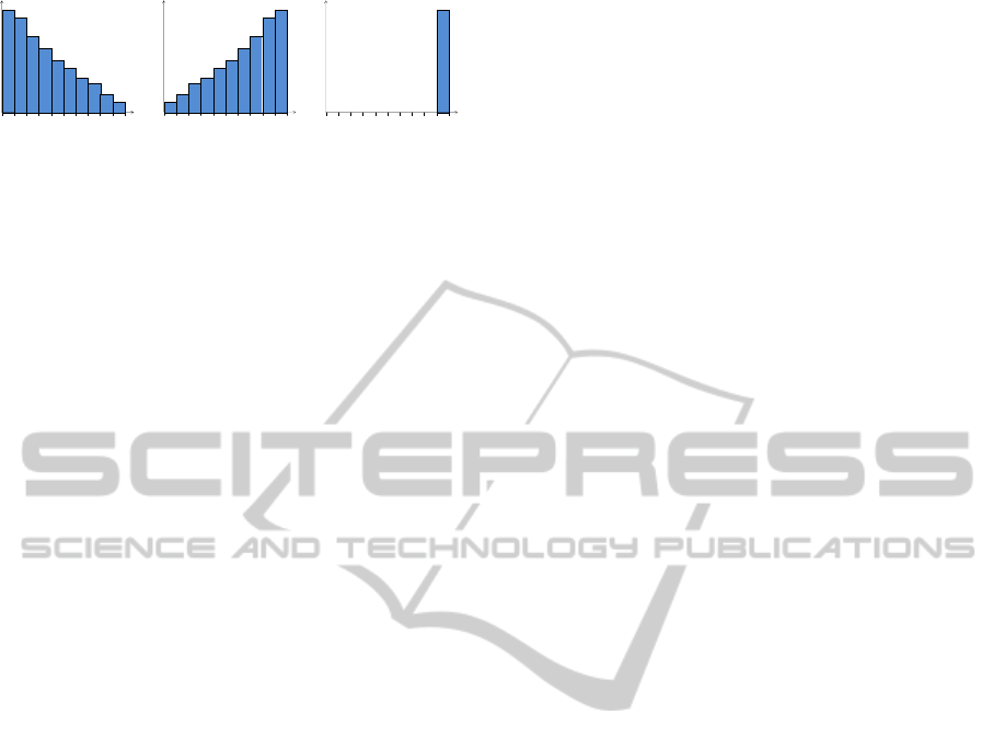
(a)
Maximum c
olor
distance
Gray distance
0
0.1
0.2
0.3
0.7
0.6
0.5
0.4
0.8
0.9
1.0
Maximum c
olor
distance
(b)
0
0.1
0.2
0.3
0.7
0.6
0.5
0.4
0.8
0.9
1.0
Gray distance
Maximum c
olor
distance
Maximum c
olor
distance
(c)
0
0.1
0.2
0.3
0.7
0.6
0.5
0.4
0.8
0.9
1.0
Gray distance
Maximum c
olor
distance
Figure 3: Pictorial representations of (a) poor, (b) good and
(c) optimal color-gray features. See text for details.
Fig. 2(b), and the color-distances that are considered
by the red outlines in Fig. 2(a). As noticed, maxi-
mum color-distance within this gray-distance interval
is 0.47, and thus is the feature value of F(8) (as shown
in Fig. 2(c)).
We note here the followings. First, a feature di-
mension corresponds to a gray-distance interval, and
a feature value to a color-distance value. In this as-
pect, the proposed color-gray feature directly incorpo-
rates both color and gray information in its represen-
tation. More importantly, each feature value indicates
the maximum color contrast of the color image that is
now represented within the currently considered gray
contrast interval, and indicates the importance of the
gray contrast interval. This information empowers us
to compute an optimal feature that retains maximum
color contrast of the color image in the form of gray
contrast, described next.
2.3 Deriving Optimal Color-gray
Feature
We seek color-gray features in which larger feature
values are present in the rightmost dimensions of the
feature. Intuitively, feature dimensions depict the ex-
tent clusters
{
c
i
}
can be distinguished in the gray
space, where larger dimensions correspond to higher
gray contrast and hence more perceivable differences
in the gray space. At the same time, a feature value
F( j) indicates the importance in the color space of the
feature dimension j, where larger feature values indi-
cate that there exist clusters which are readily distin-
guished in the color space. Thus, a color-gray feature
which has a heavy right tail corresponds to a color-to-
gray mapping in which clusters whose color contrast
are readily distinguished in the color space has gray
contrast that is easily perceived in the gray space.
Fig. 3 provides a pictorial representation of sev-
eral color-gray features. The feature of Fig. 3(a) im-
plies that clusters which are readily distinguished in
the color space (i.e. having high color contrast) are
weakly perceived in the gray space. Conversely, the
feature in Fig. 3(b) encapsulates the knowledge that
clusters which have sharp color contrast can be read-
ily distinguished in the gray space. This indicates a
better gray representation of the color clusters. By
extending this reasoning, we can derive the optimal
color-gray feature in Fig. 3(c), where regardless of
the color differences between the clusters, these clus-
ters have maximum contrast in the gray space.
2.4 Coarse-to-fine Search Strategy
We compare a color-gray feature, generated by a cur-
rent set of weight
{
w
r
, w
g
, w
b
}
and power
{
x, y, z
}
val-
ues, with the optimal feature to evaluate the quality of
the set of weight and power values. Here, we would
like to compute the minimum cost of transforming the
current color-gray feature to the optimal one. Corre-
spondingly, we employ the earth mover’s distance for
comparing between features vectors, where the fea-
ture values are normalized to sum to 1 prior to com-
puting the distance.
A na
¨
ıve method to find the best set of weight and
power values is to iterate over all values, and to se-
lect the values whose color-gray feature has the min-
imum earth mover’s distance to the optimal feature.
This however had high computational costs in the or-
der of O(n
6
). Here, we instead adopt a fast coarse-
to-fine hierarchical search strategy to find the best set
of weight/power values. Specifically, we first search
across coarse ranges of the weights values, and iden-
tify a seed weight value
{
w
r
∗
, w
g
∗
, w
b
∗
}
that has the
least earth mover’s distance from the optimal color-
gray feature. Next, we search at a finer scale in the
neighborhood of
{
w
r
∗
, w
g
∗
, w
b
∗
}
. To ensure that we
do not get trap in a local minimum, we retain three
sets of seed weight values that have the smallest earth
mover’s distances, and conduct the fine search across
the neighborhoods of these sets. At the termination of
the fine search, we identify the weight values which
have the least distance with the optimal color-gray
feature and search across various ranges of the power
values with these weight values.
The decoupling of the search for the power val-
ues from the weight values, together with the coarse-
to-fine search strategy, empowers our method with
substantial speedup over the brute force method. In
this paper, a coarse search is conducted in the range
{0, 0.2, 0.4, 0.6, 0.8, 1.0} and the fine search at an
offset of {−0.10, −0.05, 0, +0.05, 0.10} from three
sets of seed weight values. During computation, we
ignore a set of weight values if the sum of the weights
exceeds 1. The search for the power values is in the
range
{
0.25, 0.5, 0.75, 1.0
}
. The proposed method
searches over a maximum of 435 different value set-
tings, as opposed to 47439 settings using the na
¨
ıve
search method. This provides our method more than
100× speedup over the na
¨
ıve method.
ICPRAM2014-InternationalConferenceonPatternRecognitionApplicationsandMethods
456
3 RESULTS
We compare our method with Matlab’s rgb2gray
function, and recent state-of-the-art methods of (Lu
et al., 2012), (Rasche et al., 2005) and (Smith et al.,
2008). For all experiments, we evaluate the meth-
ods on the publicly available color-to-gray benchmark
dataset of (
ˇ
Cad
´
ık, 2008) which comprises 25 images.
Image decolorization by our method on all test im-
ages is achieved with the same set of parameter set-
tings, and takes under one minute per image on un-
optimized codes. We construct color-gray features
using 20 equally spaced gray intervals. Three sets
of seed weight values are computed from a coarse
intervals of {0, 0.2, 0.4, 0.6, 0.8, 1.0}. These seed
weight values are then used to initialize a fine search
at an offset of {−0.10, −0.05, 0, +0.05, 0.10}. We
find the best power values by searching across values
{0.25, 0.5, 0.75, 1.0}.
Fig. 4 show decolorization results obtained by
the proposed and comparison methods across vari-
ous synthetic and real images. We show the input
color images in the first column, and gray images
computed with Matlab’s rgb2gray function, (Lu et al.,
2012), (Rasche et al., 2005) and (Smith et al., 2008)
are shown respectively in the second to fifth columns
respectively. Gray images obtained by our method
are shown in the final column. As observed, the pro-
posed method provides perceptually more meaningful
representation of the color images, where color con-
trast present in the images are well preserved as gray
contrast. For example, consider the synthetic image
shown in the first row of Fig. 4. We note our method
to afford superior representation than existing meth-
ods, in which the contrast between the red sun and
the background is better maintained in the gray im-
age. Additionally, contrast in fine scale details cor-
responding to middle-right portion of the image are
also well preserved using our method. Decolorization
results on real images also bear out the better perfor-
mance of our method. For example, considering the
real image shown in the fifth row of Fig. 4, we note
our gray representation of the hats in the figure ren-
der them distinguishable in the gray image, and is an
improved representation over those produced by the
other methods. An interesting example is shown in
the sixth row of the figure, in which the color image
shows a green tree with small red patches on the right
side of the tree. As observed, our method is able to
generate a gray image in which red and green patches
in the color image can be distinguished by the differ-
ent gray patches in the gray image. In contrast, these
patches are indistinguishable in gray images produced
by the other comparison methods. To zoom into the
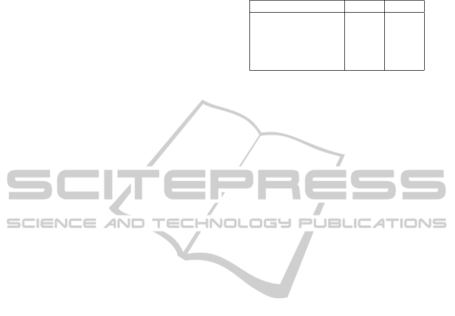
Table 1: Quantitative evaluation using color contrast pre-
serving ratio proposed by (Lu et al., 2012).
Mean Std.
Matlab rgb2gray 0.7134 0.2872
(Lu et al., 2012) 0.8213 0.1595
(Rasche et al., 2005) 0.7442 0.2565
(Smith et al., 2008) 0.8212 0.2708
Our method 0.8497 0.1621
images, please view the pdf file.
Quantitative Evaluation. We use the color contrast
preserving (CCP) ratio proposed by (Lu et al., 2012)
to quantitatively compare our methods against other
methods. This measurement evaluates the contrast
preserving ability of the methods, where larger ratios
indicate better ability to preserve color contrast in the
color image as gray contrast in the gray image. We
report the mean and standard deviation of the ratios
in Table 1. The quantities indicate our method can
satisfactorily preserve color distinctiveness and per-
form better than the other methods. A t-test shows
the comparison results to be statistically significant,
(ρ < 10
−7
).
User Study. We perform a user study to qualitatively
evaluate our method. 15 subjects with normal (or cor-
rected) vision were engaged for the study. We show
each subject a reference color image and decolorized
results obtained with the proposed and comparison
methods. To avoid bias against the methods, we ran-
domly jumbled the ordering of the gray images be-
fore presenting them to the subjects. Subjects were
instructed to identify the gray image that provides the
best representation as one in which different color
patches in the color image correspond to different
gray patches in the gray image. Overall, the subjects
identified gray images of our method as the best rep-
resentations 30.6% of the time. This compares favor-
ably to 16.0% by Matlab, 23.6% by (Lu et al., 2012),
19.3% by (Rasche et al., 2005) and 10.6% by (Smith
et al., 2008). A t-test shows the comparison results to
be statistically significant, (ρ < 10
−3
).
4 DISCUSSION
We proposed an image decolorization method that
maximally retained color contrast of a color image
as gray contrast in the resulting gray image. To-
wards this end, we proposed a novel color-gray fea-
ture which intimately couples color contrast and gray
contrast information together. This feature provides
us with a unique advantage to directly evaluate the
quality of a gray image based on information avail-
ImageDecolorizationbyMaximallyPreservingColorContrast
457
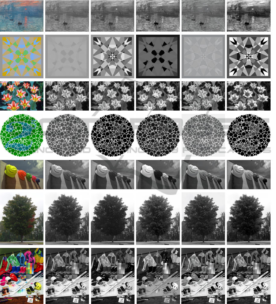
Figure 4: Decolorization results. First column shows reference color image. Gray images obtained with Matlab’s rgb2gray
function, (Lu et al., 2012), (Rasche et al., 2005) and (Smith et al., 2008) are shown respectively in the second to fifth columns.
Final column shows gray images obtained with our method. This figure is best viewed with magnification.
able in the color image. More importantly, it also af-
fords us with a mechanism to drive our search to find
the best color-to-gray decolorization function which
maximally preserves contrast in the gray image. Here,
a non-linear decolorization function is employed to
convert a color image to its gray representation, in
which we reduce computation cost by a coarse-to-fine
search strategy. We show through experimental com-
parisons and user study the greater effectiveness of
our approach. As future work, we are interested to
extend our method to decolorize movie frames, where
we will exploit both spatial and temporal cues to en-
ICPRAM2014-InternationalConferenceonPatternRecognitionApplicationsandMethods
458

sure coherency in gray representation is maintained
across different movie frames.
REFERENCES
Bala, R. and Eschbach, R. (2004). Spatial color-to-
grayscale transform preserving chrominance edge in-
formation. Color Imaging Conference, pages 82–86.
ˇ
Cad
´
ık, M. (2008). Perceptual evaluation of color-to-
grayscale image conversions. Comput. Graph. Forum,
27(7):1745–1754.
Cheng, Y. (1995). Mean shift, mode seeking, and clustering.
IEEE Transactions on Pattern Analysis and Machine
Intelligence, 17(8):790–799.
Gooch, A., Olsen, S., Tumblin, J., and Gooch, B. (2005).
Color2gray: Salience-preserving color removal. ACM
Transactions on Graphics, 24(3):634–639.
Kim, Y., Jang, C., Julien, J., and Lee, S. (2009). Ro-
bust color-to-gray via nonlinear global mapping. ACM
Transactions on Graphics, 28(5).
Lu, C., Xu, L., and Jia, J. (2012). Realtime contrast pre-
serving decolorization. ACM SIGGRAPH Asia.
MATLAB (2010). version 7.10.0 (r2010a).
Neumann, L., Cadik, M., and Nemcsics, A. (2007). An ef-
ficient perception-based adaptive color to gray trans-
formation. Proc. of Comput. Aesthetics, pages 73–80.
Rasche, K., Geist, R., and Westall, J. (2005). Re-coloring
images for gamuts of lower dimension. Computer
Graphics Forum, pages 423–432.
Smith, K., Landes, P., Thollot, J., and Myszkowski, K.
(2008). Apparent greyscale: A simple and fast conver-
sion to perceptually accurate images and video. Com-
puter Graphics Forum, pages 193–200.
ImageDecolorizationbyMaximallyPreservingColorContrast
459
