
Research Proposal in Probabilistic Planning Search
Yazmin S. Villegas-Hernandez and Federico Guedea-Elizalde
Design and Technology Innovation Center, Tecnologico de Monterrey, Monterrey, Mexico
Keywords:
Bayesian Networks, Planning, and Planning Search.
Abstract:
In planning search, there are different approaches to guide the search, where all of them are focused in have a
plan (solution) in less time. Most of the researches are not admissible heuristics, but they have good results in
time. For example, using the heuristic-search planning approach plans can be generated in less time than other
approaches, but the plans generated by all heuristic planners are sub-optimal, or could have dead ends (states
from which the goals get unreachable). We present an approach to guide the search in a probabilistic way in
order to do not have the problems of the not admissible approaches. We extended the Bayesian network and
Bayesian inferences ideas to our work. Furthermore, we present our way to make Bayesian inferences in order
to guide the search in a better way. The results of our experiments of our approach with different well-known
benchmarks are presented. The benchmarks used in our experiments are: Driverlog, Zenotravel, Satellite,
Rovers, and Freecell.
1 INTRODUCTION
In planning, there are four main approaches to in-
crease the efficiency of planning systems.
First, Blum and Furst developed a novel algorithm
called Graphplan (Blum and Furst, 1997). This al-
gorithm reduces the branching factor by searching in
a special data structure. Furthermore, this algorithm
searches for layered plans (parallel plans). This algo-
rithm has three limitations. First, Graphplan applies
only to STRIPS language (Fikes and Nilsson, 1994).
Second, this planner performs poorly without extra ad
hoc reasoning capabilities. Third, the most important
limitation of Graphplan is that the quality of the plan
is not as good as the speed of the planning of this
planner.
There are many planning systems that use the
Graphplan algorithm or their own version of this al-
gorithm as SGP (Weld et al., 1998), Blackbox (Kautz
and Selman, 1999), IPP (Koehler, 1999), Medic
(Ernst et al., 1997), STAN (Fox and Long, 2011),
FF (Hoffmann and Nebel, 2011) and others. Further-
more, there is the LPG (Local Search for Planning
Graphs) planner (Gerevini et al., 2003), which is the
only one that does not use the Graphplan algorithm
properly, but it still has a planning-graph approach.
Therefore, LPG works with heuristics that exploit the
structure of the planning graph.
Second, Kautz and Selman developed a novel
method for planning called planning as satisfiability
(SAT) (Kautz et al., 1992), which transforms plan-
ning problem into a propositional satisfiability prob-
lem for which efficient solvers are known. The SAT-
PLAN04 (Kautz, 2004) uses STRIPS language as
well as PDDL language (Fox and Long, 2003), but
SatPlan does not handle any non-STRIPS features
other than types, such as derived effects and condi-
tional actions.
Third, Bonet and Geffner developed a new ap-
proach based on heuristic-search planning (HSP)
(Bonet and Geffner, 2001). In this approach, a heuris-
tic is choosing among a set of different heuristics in
order to guide the search through the state space. Un-
fortunately, the heuristics used in this algorithm are
not fully admissible. Indeed, these heuristics do not
work for all domains.
Hoffman and Nebel, using and improving HSP
ideas, developed the FF (Fast-Forward) system (Hoff-
mann and Nebel, 2011), which is one of the fastest
planners in STRIPS language. The FF heuristic im-
plements a relaxed Graphplan algorithm to obtain the
minimum distance between the state and the goal
state, but this relaxed algorithm is not admissible be-
cause the relaxed Graphplan not consider the delete
list (which is all the delete effects of all operators).
The search algorithm, called Enforced Hill-Climbing
(EHC), only does a local search, which can lead to
dead ends (states from which the goals get unreach-
able).
Fourth, Bonet and Geffner used and improved
586
S. Villegas-Hernandez Y. and Guedea-Elizalde F..
Research Proposal in Probabilistic Planning Search.
DOI: 10.5220/0004907205860595
In Proceedings of the 6th International Conference on Agents and Artificial Intelligence (ICAART-2014), pages 586-595
ISBN: 978-989-758-015-4
Copyright
c
2014 SCITEPRESS (Science and Technology Publications, Lda.)

ideas of planning with incomplete information (Gene-
sereth and Nourbakhsh, 1993) to develop another
approach based on planning with incomplete infor-
mation as heuristic search in belief space (Geffner,
2011).
Planning with incomplete information is distin-
guished from classical planning in the type and
amount of information available at planning and exe-
cution time. In planning with incomplete information,
the initial state is not known, but sensor information
may be available at execution time. By contrast, in
classical planning the initial state is known and there
is no sensor to get knowledge or feedback of the states
at execution time.
Planning with incomplete information can be for-
mulated as a problem of search in belief space, where
belief states can be either set of states or more gen-
erally probability distribution over states. Bonet and
Geffner made the explicit formulation of planning
with incomplete information, in order to extend it
to tasks like contingent planning where the standard
heuristic search algorithms do not apply. The limita-
tions of this planner are two. The first limitation is
that the search algorithm is not optimal like A*. The
second limitation is the complexity of a number of
preprocessing and runtime operations in GPT (Gen-
eral Planning Tool) (Bonet and Geffner, 2011) scales
with the size of the state space.
The heuristic-search planning approach has good
results in execution time, but the plans generated by
all heuristic planners are sub-optimal, or could have
dead ends (states from which the goals get unreach-
able). Our approach is different from heuristic-search,
we developed a probabilistic method to guide the
search in an efficient way, in order to not have dead
ends, and also have optimal plans.
The paper is organized as follows. First, we ex-
plain classical planning, Bayesian inference and the
probabilistic planning search. Then we report results
of the experiments and some conclusions are drawn.
2 CLASSICAL PLANNING
FRAMEWORK
In Classical Planning (Russell, 2009), there are only
considered environments that are fully observable, de-
terministic, finite, static (change happens only when
the agent acts), and discrete (in time, action, objects,
and effects).
Classical Planning (Nilsson, 2010) is defined as
a tuple
∑
=< S, S
0
, S
G
, A >, where S is a finite state
space, S
0
is an initial situation given by a single state
S
0
∈ S, S
G
is a goal situation given by a non-empty
set of states S
G
⊆ S, and A is a set of finite actions.
These actions A(s) ⊆ A are applicable in each state
s ∈ S, and every action a ∈ A(s) maps each state s ∈ S
into another state s
a
= f (a, s) in a deterministic way.
Indeed, there are positive action costs c(a, s) for doing
an action a ∈ A(s) in a state s ∈ S.
A plan (solution) for a deterministic problem is
a sequence of actions {a
0
, a
1
, . . . , a
k
} that generates
a state trajectory {s
0
, s
1
= f (s
0
), . . . , s
k+1
= f (s
i
, a
i
)}
such that each action a
i
∈ A(s
i
) is applicable in state
s
i
∈ S and s
k+1
∈ S
G
is a goal state. A plan π is opti-
mal when the total cost
∑
k
i=0
c(s
i
, a
i
) ≥ 0 of doing an
action a
i
∈ A(s) in a state s
i
∈ S is minimal.
In Classical Planning is used a transition function
f (s
i
, s
i+1
, a
i
) to guide the search (from a state s
i
to an-
other state s
i+1
using an action a
i
) to reach a solution.
The most successful planners use heuristics to have a
solution in less time as do FF, HSP, and others. But,
these planners do not have the same results in length
(of the solution) as in time. In order to deliver bet-
ter results in length, we propose a novel approach
to guide the search in Planning using Bayesian infer-
ence.
3 BAYESIAN NETWORK AND
INFERENCE
Bayesian networks (Russell, 2009) are directed
acyclic graphs whose events (nodes) are represented
by random variables which can have several states
with a probability of happening.
Figure 1 depicts a Bayesian network (Russell,
2009) where an event has an effect in several events,
and one or more events can have an effect on one
event.
Figure 1: Bayesian network.
Bayesian Inference (O’Hagan et al., 2004) is a
method of inference that update the probability of a
hypothesis (belief) using Bayes’ rule as additional ev-
idence is acquired.
ResearchProposalinProbabilisticPlanningSearch
587

The process of inference has two steps:
1. Update of the belief given an evidence
2. Propagation of the evidence through the network
Morawski defined a novel model of Bayesian net-
work, which consists of a tree with one father with
several children in a hierarchical way (Morawski,
1989). Indeed, the tree has a father-children relation-
ship, where the father sends information to his son
(π) and a son to his father (λ). Figure 2 depicts the
Morawski model of a Bayesian network.
Figure 2: Evidence propagation in a bayesian network.
In this cause-effect relationship between father
and children we have both evidence: diagnostic and
causal evidence, where these evidences use the chain
rule given conditional independence to be estimated.
Furthermore, we have a node belief which uses the
causal and diagnostic evidence.
Diagnostic evidence is estimated, in equation 1,
using λ information of an event. In this expression,
Children( f
i
) stands for the children of the event (fa-
ther node) f
i
and λ
k
( f
i
) stands for the probability of
an event k happening given the event (father node) f
i
,
which is sent from the event k to the event f
i
. .
λ( f
i
) =
∏
k∈Children( f
i
)
λ
k
( f
i
) (1)
Causal evidence, which is defined in equation 2,
uses π information of an event. Furthermore, this
evidence is estimated using the conditional indepen-
dence and rule chain. In this expression, s
i
stands for
a state of the event S, States( f ) stands for the states
of the event f , P(s
i
| f
k
) stands for the probability of
happening state s
i
given his father(s) f
k
, π
S
( f
k
) stands
for the probability of happening the event f
k
sent from
the event f
k
to the event S, and f ather(S) stands for
the fathers of the event S.
π(s
i
) =
∑
k∈States( f )
P(s
i
| f
k
)
∏
f ∈ f ather(S)
π
S
( f
k
) (2)
The belief of an event e
i
is estimated, in equation
3, using the λ and π information (of his son and fa-
ther), where α is a normalization constant to maintain
in balance the joint probabilities, i.e. to maintain the
sum of all beliefs (in a Bayesian network) equal to 1.
β(e
i
) = απ(e
i
)λ(e
i
) (3)
Bayesian inference is used to do inference be-
tween conditional events, which could be helpful in
a planning problem search to reach to an optimal so-
lution in a probabilistic way.
4 PROPOSAL PROBABILISTIC
PLANNING
We propose a novel Probabilistic Planning Search,
which introduces the use of probability to guide the
search space in a non-relaxed way. Furthermore,
we propose a model for planning with probabilistic
search where a goal is achieved taking account the
probability to reach a goal state.
The model for the probabilistic planning is char-
acterized by a quintuple
∑
=< S, S
0
, S
G
, A, P > where
S is a finite state space, S
0
is a non-empty set of possi-
ble initial states S
0
∈ S, S
G
is a non-empty set of goal
states, A is a set of actions with A(s) denoting the ac-
tions applicable in state s A(s) ∈ A, and P is a proba-
bility transition function such that P(s
k
|a
i
, s
i
) denotes
the non-empty set of probabilities of passing from the
an initial state s
i
using an action a
i
to the state s
k
.
In our approach we try to establish a basic form
to search in the Bayesian network using Morawski
model. We defined the causal and diagnostic evidence
based on the amount of children states and on the dis-
tance from this state to the goal, respectively. Intu-
itively, we reduce the branch factor with the causal
evidence because it takes account the less amount of
children states; and reduce the plan length because
we take account the minimum cost to reach the goal.
This probability transition function is used to guide
the search, where the maximum probability is chosen
in each state.
ICAART2014-InternationalConferenceonAgentsandArtificialIntelligence
588

4.1 Bayesian Inference
The state space, where nodes are states, can be mod-
eled as a Bayesian network (with a father-children
structure) with events replaced by states s ∈ S and
arrows (which establish cause-effect relationship be-
tween events) are replaced by actions a ∈ A(s).
Morawski used the belief equation of an event e
i
to estimate the probability of this event e
i
given other
events that occur in the past. In the same way, we use
this belief equation to estimate the probability to find
the goal state g ∈ S given an action a ∈ A(s) chosen a
shorter way. In this probabilistic model, we estimate
the probability transition function as equation 4.
P(s
k
|a
i
, s
i
) = αλ
children(s
i
,a
i
)
(s
k
)π
s
i
(s
k
) (4)
In these expressions, λ
children(s
i
,a
i
,)
(s
k
) stands
for the probability of happening of the son state
children(s
i
, a
i
) given the state s
k
, π
s
i
(s
k
) stands for the
probability of happening s
k
, and α is a normalization
constant to maintain the sum of the total probability
equal to 1.
The probability transition function estimates the
shorter branching factor to reach a goal state. This
equation uses causal and diagnostic evidence. These
evidences can be estimated using cost equations of
reaching the goal state and branching.
c(g;s) :=
0 g ∈ s
min
a∈A(s)
[1 + c(s
prec
;s)] otherwise
(5)
The main costs used to update the probabil-
ity transition function are the maximum and total
cost. For the estimation of these costs, we used the
Bellman-Ford algorithm (Vector, 2003), equation 5,
to estimate the shorter length cost to reach a goal state
g ∈ S from state s ∈ S. In this expression, s
prec
stands
for the precondition states (or prior states).
For the estimation of the total cost of the branch-
ing factor, in equation 6, it is defined as the sum of
the costs c(g
i
, s) of each goal state g
i
∈ G, where G
stands for the set of goal states G ∈ S.
c
total
(G;s) :=
∑
g
i
∈G
c(g
i
;s) (6)
The estimation of the maximum cost of branching
factor, in equation 7, is defined as the maximum cost
c(g
i
, s) of each goal state g
i
∈ G.
c
max
(G;s) := max
g
i
∈G
[c(g
i
;s)] (7)
The estimation of λ
s
i
(¬s
k
), which is the probabil-
ity of not happening the state s
i
(in a shorter way)
given the goal state s
k
, is defined as equation 8. We
divided the maximum cost of branching factor by the
total cost of branching factor, because it represents the
largest-search-cost possibility divided by all possibil-
ities.
λ
s
i
(¬s
k
) =
c
max
(s
k
;s
i
)
c
total
(s
k
;s
i
)
(8)
The complement of λ
s
i
(¬s
k
) is λ
s
i
(s
k
), which is
estimated as equation 9.
λ
s
i
(s
k
) = 1 − λ(¬s
k
) (9)
The estimation of π
s
i
(¬s
k
), which is the probabil-
ity of not happening state s
k
in a shorter way, is in
equation 10. In this expression, Children(s
i
) stands
for the son states of the state s
i
.
π
s
i
(¬s
k
) =
1
Children(s
i
)
(10)
The complement of π
s
i
(¬s
k
) is π
s
i
(s
k
), which is
estimated in equation 11.
π
s
i
(s
k
) = 1 −
1
Children(s
i
)
(11)
Both equations (9) and (11) are used to esti-
mate the probability of the shorter branching fac-
tor of a state space (modeled as Bayesian network).
Therefore, using our approach, we would expect that
shorter plans can be found compared with a heuris-
tic approach. We discuss below the results of our
approach in different domains compared with other
planner approaches.
5 EXPERIMENTS & RESULTS
We compared the performance of our approach
with other planner approaches for some well-known
benchmark problems (STRIPS like) of the AIPS-2002
competition set. We considered Blackbox, which is
the combination of both approaches Graphplan and
SAT; HSP, which uses the heuristic approach; Metric-
ff, which uses and improved the same ideas from HSP
approach; and LPG, which is a planning-graph ap-
proach (which is different to Graphplan algorithm, but
it used in this planner the same graph-search idea).
Furthermore, all the experiments of our probabilistic
approach where using a backward approach and the
Breadth-first search algorithm.
For each benchmark, it was estimated for each
approach the mean percentage error (MPE) between
ResearchProposalinProbabilisticPlanningSearch
589
the plan-length results of such approach and the plan-
length minimum of all approaches in each instance.
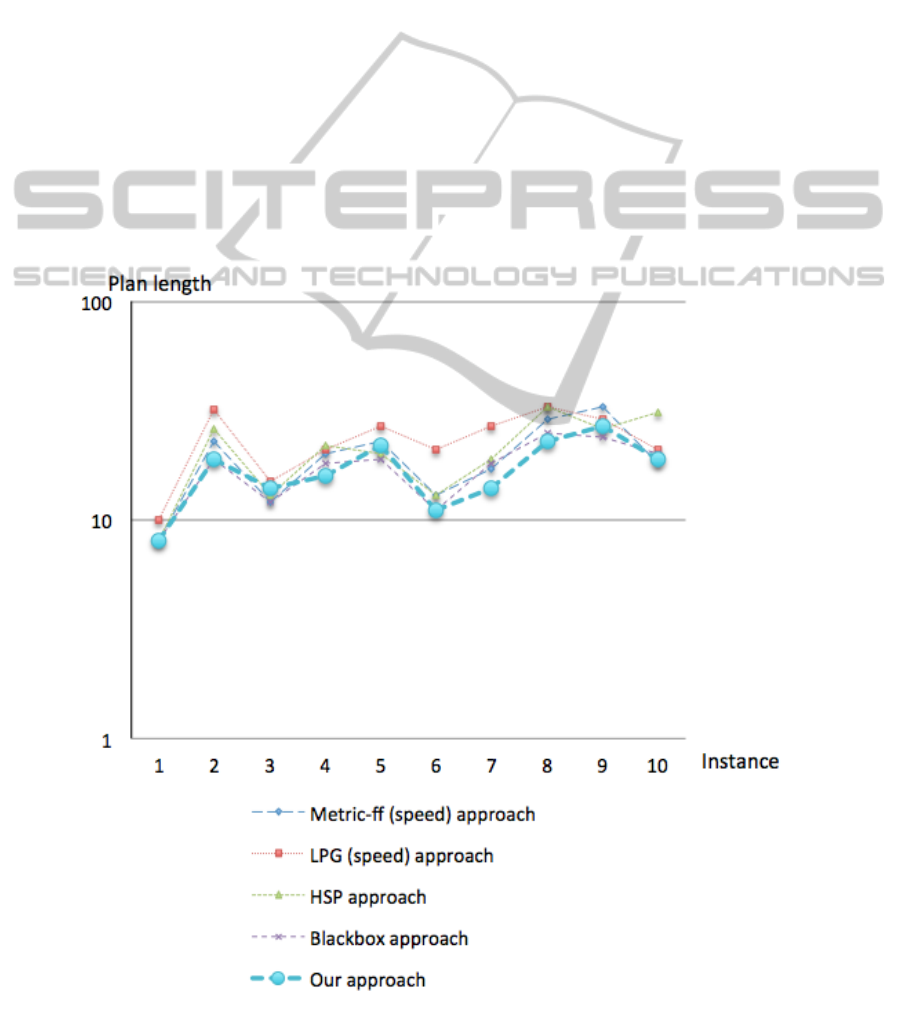
5.1 Driverlog Benchmark
The Driverlog domain is a variation of Logistics
where the trucks need drivers, furthermore some paths
can only be traversed by truck, and others only on
foot.
Figure 3 depicts the plan-length curves (in loga-
rithmic scale with base 10) on Driverlog instances,
which their size scales from left to right.
Our approach, in these Driverlog instances, solved
most of the problems with less steps in the plan (so-
lution). Our approach dominates both approaches
LPG and HSP. Only in few instances both Blackbox
and Metric-ff (in speed version) obtained better plan-
length results.
In terms of mean percentage error (MPE), our ap-
proach has less error than the other approaches. In
comparison with the best results for each approach,
our approach has 0.050 of MPE, Blackbox has 0.060
of MPE, Metric-ff has 0.163, HSP has 0.297, and
LPG has 0.436 of MPE.
5.2 Zenotravel Benchmark
The Zenotravel domain is a transportation problem,
where objects must be transported by airplanes, and
each airplane has an associated fuel level.
Figure 4 depicts the plan-length curves (in loga-
rithmic scale with base 10) on Zenotravel instances,
which their size scales from left to right.
Metric-ff approach and our approach solved the
Zenotravel instances in less steps than the others, but
Metric-ff cannot perform one instance in this domain.
Furthermore, the Blackbox approach can give a so-
lution to any instance in this domain. Only in three
instances our approach has equal or better results in
comparison with Metric-ff approach.
In terms of mean percentage error (MPE), Metric-
ff and our approach have less error than the other ap-
Figure 3: Plan-length curves on Driverlog instances.
ICAART2014-InternationalConferenceonAgentsandArtificialIntelligence
590
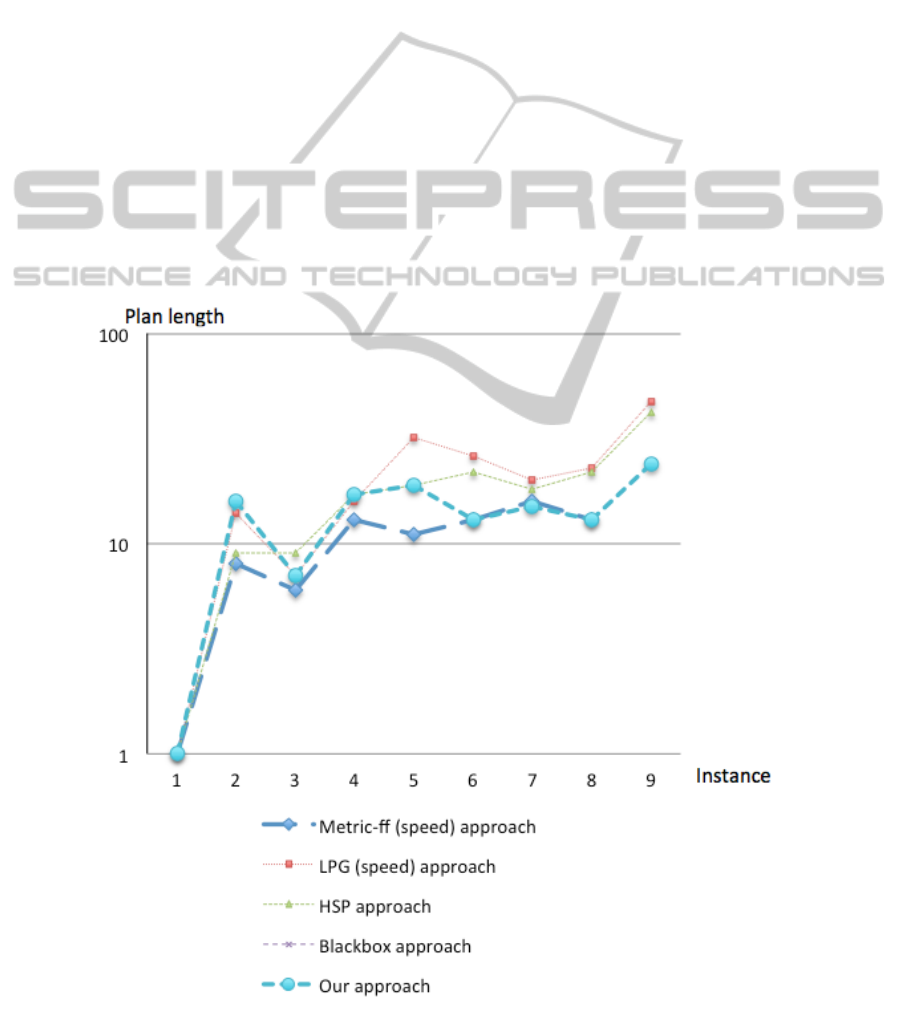
proaches. In comparison with the best results for each
approach, Metric-ff has 0.118 of MPE, our approach
has 0.224 of MPE, HSP has 0.443, LPG has 0.679 of
MPE, and Blackbox cannot perform any instance in
this domain.
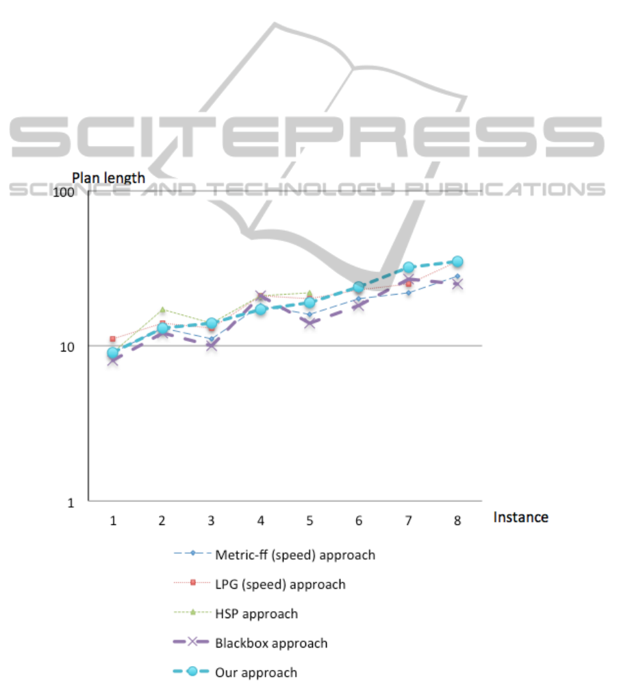
5.3 Satellite Benchmark
In Satellite domain, a number of satellites must take
some observations using some instruments. The ac-
tions that a satellite can do are turning in the right
direction, switching the instruments on or off, cali-
brating the instruments, and taking images.
Figure 5 depicts the plan-length curves (in log-
arithmic scale with base 10) on Satellite instances,
which their size scales from left to right.
In terms of mean percentage error (MPE), Black-
box Metric-ff and our approach have less error than
the other approaches. In comparison with the best re-
sults for each approach, Blackbox has 0.057 of MPE,
Metric-ff has 0.092 of MPE, our approach has 0.269
of MPE, LPG has 0.289 of MPE, and HSP has 0.593.
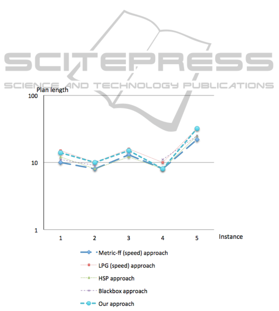
5.4 Rovers Benchmark
In Rovers domain, a number of planetary rovers must
analyze some samples, and take images. The actions
of a rover include navigating, taking samples, cali-
brating the camera and taking images, and communi-
cating the data.
Figure 6 depicts the plan-length curves (in log-
arithmic scale with base 10) on Rovers instances,
which their size scales from left to right.
In this domain, Metric-ff, HSP and our approach
have a better performance than the other approaches.
Metric-ff and HSP weakly dominates our approach
having equal or better results.
In terms of mean percentage error (MPE), Metric-
ff, HSP and our approach have less error than the
other approaches. In comparison with the best results
for each approach, Metric-ff has 0.016 of MPE, HSP
has 0.067, our approach has 0.270 of MPE, Blackbox
has 0.347, and LPG has 0.357 of MPE.
Figure 4: Plan-length curves on Zenotravel instances.
ResearchProposalinProbabilisticPlanningSearch
591
5.5 Freecell Benchmark
The Freecell domain is a well-known domain of dis-
crete puzzles, where all cards are randomly divided
into a number of piles. The objective of the game is
to move all cards onto four different piles for each
suit, where the cards are arranged upwards from the
ace to the king.
Figure 7 depicts the plan-length curves (in log-
arithmic scale with base 10) on Freecell instances,
which their size scales from left to right.
In this domain, both LPG and HSP approaches do
not have a solution for all tested instances, and it is
not clear which approach is best.
In terms of mean percentage error (MPE), Metric-
ff and our approach have less error than the other ap-
proaches. In comparison with the best results for each
approach, Metric-ff has 0.083 of MPE, our approach
has 0.166 of MPE, HSP has 0.38 of MPE, LPG has
0.517 of MPE, and Blackbox has 0.526.
5.6 Overall Results
Metric-ff and our approach have the best performance
in all the domains tested. Therefore, they have less
mean percentage error in plan-length results in gen-
eral.
Our probabilistic approach has better results than
Blackbox (which is the combination of Graphplan and
Sat approach), LPG (planning-graph approach), HSP
(heuristic-search approach), but our approach cannot
have overall better results in comparison with Metric-
ff (a heuristic approach that uses a relaxed Graphplan
algorithm as a heuristic and a novel Enforced Hill
Climbing search algorithm).
Our approach, as the other approaches, has diffi-
culties to work with complex problems (i.e. domains
with many actions, predicates, objects and goals). In
our experiments, the complexity level of each well-
known benchmark is increased, where we can see that
the level of complexity depends on the benchmark
Figure 5: Plan-length curves on Satellite instances.
ICAART2014-InternationalConferenceonAgentsandArtificialIntelligence
592
used.
6 CONCLUSIONS
We have presented and modeled a novel probabilis-
tic planning search approach. This probabilistic have
good results in comparison with the other approaches.
The most important contribution is the “probabilistic
search approach” idea.
We extended the Bayesian network idea to state
space. The state space was modeled as a father-
children network structure. Using this network we
could make inferences using our Bayesian inference
equations.
Furthermore, we defined explicitly probabilistic
functions in order to define the Bayesian inference
equations, which are based on well-known rules as
both Bayes’ rule and conditional independence.
In our experiments with different benchmarks we
found that our approach have good results in terms of
plan length.
Our future work focus on the search algorithm
that works better with our Bayesian inferences in or-
der to get optimal results, which means to have plans
with less length in less time.
The benchmarks have different variables (states),
which have an influence on data distribution. Indeed,
this affects our Bayesian inferences, in order to have
better results in our future work we will study the data
distribution of different well-known benchmark and
we will determine the Bayesian inference equations
that work best with.
ACKNOWLEDGEMENTS
This research was supported by ITESM under the Re-
search Chair CAT-100.
Figure 6: Plan-length curves on Rovers instances.
ResearchProposalinProbabilisticPlanningSearch
593
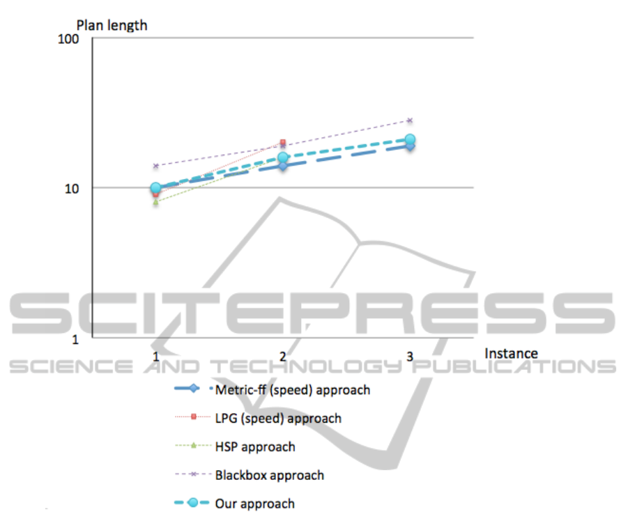
Figure 7: Plan-length curves on Freecell instances.
REFERENCES
Blum, A. L. and Furst, M. L. (1997). Fast planning
through planning graph analysis. Artificial intelli-
gence, 90(1):281–300.
Bonet, B. and Geffner, H. (2001). Planning as heuristic
search. Artificial Intelligence, 129(1):5–33.
Bonet, B. and Geffner, H. (2011). mgpt: A probabilis-
tic planner based on heuristic search. arXiv preprint
arXiv:1109.2153.
Ernst, M. D., Millstein, T. D., and Weld, D. S. (1997). Auto-
matic sat-compilation of planning problems. In IJCAI,
volume 97, pages 1169–1176. Citeseer.
Fikes, R. E. and Nilsson, N. J. (1994). Strips, a retrospec-
tive. Artificial intelligence in perspective, 227.
Fox, M. and Long, D. (2003). Pddl2. 1: An extension to
pddl for expressing temporal planning domains. J. Ar-
tif. Intell. Res.(JAIR), 20:61–124.
Fox, M. and Long, D. (2011). Efficient implementa-
tion of the plan graph in stan. arXiv preprint
arXiv:1105.5457.
Geffner, H. (2011). Planning with incomplete information.
In Model Checking and Artificial Intelligence, pages
1–11. Springer.
Genesereth, M. and Nourbakhsh, I. (1993). Time-saving
tips for problem solving with incomplete information.
In Proceedings of the 11th National Conference on Ar-
tificial Intelligence.
Gerevini, A., Saetti, A., and Serina, I. (2003). Planning
through stochastic local search and temporal action
graphs in lpg. J. Artif. Intell. Res.(JAIR), 20:239–290.
Hoffmann, J. and Nebel, B. (2011). The ff planning system:
Fast plan generation through heuristic search. arXiv
preprint arXiv:1106.0675.
Kautz, H. (2004). Satplan04: Planning as satisfiability.
Working Notes on the Fourth International Planning
Competition (IPC-2004), pages 44–45.
Kautz, H. and Selman, B. (1999). Unifying sat-based and
graph-based planning. In IJCAI, volume 99, pages
318–325.
Kautz, H. A., Selman, B., et al. (1992). Planning as satisfi-
ability. In ECAI, volume 92, pages 359–363.
ICAART2014-InternationalConferenceonAgentsandArtificialIntelligence
594

Koehler, J. (1999). Handling of conditional effects and neg-
ative goals in ipp.
Morawski, P. (1989). Understanding bayesian belief net-
works. AI Expert, 4(5):44–48.
Nilsson, N. J. (2010). The quest for artificial intelligence.
Cambridge University Press Cambridge.
O’Hagan, A., Forster, J., and Kendall, M. G. (2004).
Bayesian inference. Arnold London.
Russell, S. (2009). Artificial intelligence: A modern ap-
proach.
Vector, D. (2003). Routing. Perkins, E. Royer.
Weld, D. S., Anderson, C. R., and Smith, D. E. (1998). Ex-
tending graphplan to handle uncertainty & sensing ac-
tions. In Aaai/iaai, pages 897–904.
ResearchProposalinProbabilisticPlanningSearch
595
