Episode Rules Mining Algorithm for Distant Event Prediction
Lina Fahed, Armelle Brun and Anne Boyer
Universit´e de Lorraine, LORIA,
´
Equipe KIWI, Campus Scientifique, BP 239 54506, Vandoeuvre-l`es-Nancy Cedex, France
Keywords:
Data Mining, Episode Rules Mining, Minimal Rules, Distant Event Prediction.
Abstract:
This paper focuses on event prediction in an event sequence, where we aim at predicting distant events. We
propose an algorithm that mines episode rules, which are minimal and have a consequent temporally distant
from the antecedent. As traditional algorithms are not able to mine directly rules with such characteristics,
we propose an original way to mine these rules. Our algorithm, which has a complexity similar to that of
state of the art algorithms, determines the consequent of an episode rule at an early stage in the mining
process, it applies a span constraint on the antecedent and a gap constraint between the antecedent and the
consequent. A new confidence measure, the temporal confidence, is proposed, which evaluates the confidence
of a rule in relation to the predefined gap. The algorithm is validated on an event sequence of social networks
messages. We show that minimal rules with a distant consequent are actually formed and that they can be used
to accurately predict distant events.
1 INTRODUCTION
The flow of messages posted in blogs and social net-
works is an important and valuable source of infor-
mation that can be analyzed, modeled (through the
extraction of hidden relationships) and from which in-
formation can be predicted, which is the focus of our
work. For example, companies may be interested in
the prediction of what will be said about them in so-
cial networks. Similarly, this prediction can be a way
to recommend items. We consider that the sooner an
event is predicted, the more useful this prediction is
for the company or the person concerned, since this
allows to have enough time to act before the occur-
rence of the event. Predicting distant events is thus
the focus of our work.
Temporal data mining is related to the mining
of sequential patterns ordered by a given criterion
such as time or position (Laxman and Sastry, 2006).
Episode mining is the appropriate pattern discovery
task related to the case the data is made up of a sin-
gle long sequence. An episode is a temporal pattern
made up of “relatively close” partially ordered items
(or events), which often appears throughout the se-
quence or in a part of it (Mannila et al., 1997). When
the order of items is total, the episode is said to be se-
rial. Similarly to the extraction of association rules
from itemsets, episode rules can be extracted from
episodes to predict events (Cho et al., 2011). The
rule mining task is usually decomposed into two sub-
problems. The first one is the discovery of frequent
itemsets or episodes that have a support higher than a
predefined threshold. The second one is the genera-
tion of rules from those frequent itemsets or episodes,
with the constraint of a minimal confidence thresh-
old (Agrawal et al., 1993). In general, rules are gen-
erated by considering some items in the itemset (or
the last items in the episode) as the consequent of the
rule, and the rest of the items as the antecedent. Since
the second sub-problem is quite straightforward, most
of the researches focus on the first one: the extraction
of itemsets or episodes.
Episode and episode rules mining are used in
many areas, such as telecommunication alarm man-
agement (Mannila et al., 1997), intrusion detec-
tion (Luo and Bridges, 2000), discovery of relation
between financial events (Ng and Fu, 2003), etc.
Our goal is to reliably predict events that will oc-
cur after a predetermined temporal distance, in order
to have enough time to act before the occurrence of
events. Therefore, serial episode rules with a conse-
quent distant from the antecedent will be mined. Tra-
ditional episode rules mining algorithms form episode
rules with a consequent close to the antecedent. To
mine rules with a distant consequent, these algorithms
have to perform a post-processing step: the extracted
rules are filtered to keep only rules with a consequent
that may occur far from the antecedent. This post-
5
Fahed L., Brun A. and Boyer A..
Episode Rules Mining Algorithm for Distant Event Prediction.
DOI: 10.5220/0005027600050013
In Proceedings of the International Conference on Knowledge Discovery and Information Retrieval (KDIR-2014), pages 5-13
ISBN: 978-989-758-048-2
Copyright
c
 2014 SCITEPRESS (Science and Technology Publications, Lda.)

processing is not only time consuming, but also the
time required for mining rules which will be filtered
out is useless. Thus, we propose a new algorithm for
mining serial episode rules, with a consequent tem-
porally distant from the antecedent, to predict dis-
tant events, and with a small antecedent (in number
of events and in time), to be able to predict events
as soon as possible. This algorithm has a complexity
equal to that of traditional algorithms.
An example of a required rule is presented be-
low (from a sequence of annotated messages of blogs
about finance issues, where each event includes a sen-
timent polarity): R: (interest rate, neutral) (credit,
negative) (waiting, neutral) → (concurrence, nega-
tive); the antecedent occurs within 5 days, the gap
between the antecedent and the consequent is 15 days.
The rest of this paper is organized as follows: sec-
tion 2 presents related works about episode rules min-
ing. Our algorithm is introduced in section 3, fol-
lowed by experimental results in section 4. We con-
clude and provide some perspectives in section 5.
2 RELATED WORKS
We first start by introducing few concepts. Let I =
{i
1
,i
2
,...,i
m
} be a finite set of items. I
t
is the set of
items that occur at a timestamp t referred to as an
event. An event sequence S is an ordered list of
events, S =< (t
1
,I
t
1
),(t
2
,I
t
2
),...,(t
n
,I
t
n
) > with t
1
<
t
2
< ... < t
n
, (see Figure 1). The serial episode P =<
p
1
, p
2
,..., p
k
> on I
k
is an ordered list of events. Its
support, denotedto as supp(P), representsthe number
of occurrences of P, according to a frequency mea-
sure. P is said to be a frequent episode if supp(P) ≥
minsupp where minsupp is the predefined minimal
threshold. An occurrence window of the episode P
is a segment < I
t
s
,...,I
t
e
> of the sequence, denoted as
OW(S,t
s
,t
e
) which starts at timestamp t
s
and ends at
timestamp t
e
, where P ⊆< I
t
s
,...,I
t
e
>, p
1
⊆ I
t
s
and
p
k
⊆ I
t
e
. It represents the interval that bounds the
episode. Let P,Q be two episodes. An episode rule
R : P → Q means that Q appears after P. The con-
fidence of this episode rule is the probability to find
Q after P: conf(P → Q) = supp(P.Q)/supp(P). The
rule is said to be confident if its confidence exceeds a
predefined threshold minconf .
Winepi and Minepi are seminal episode mining
algorithms (Mannila et al., 1997), and are the basis
of many other algorithms. To extract episodes, both
algorithms start by extracting 1-tuple episodes (made
up of one item), then iteratively seek larger ones by
merging items on their right side. This approach is
the one used by many other algorithms (Laxman et al.,
2007) (Huang and Chang, 2008).
In the frequent itemsets mining task (which in-
cludes episode mining), it is suggested that anti-
monotonicity is a common property that has to be re-
spected by any frequency measure (Agrawal et al.,
1993). Several frequency measures for episode min-
ing have been proposed. In (Mannila et al., 1997),
window-based and minimal occurrence-based fre-
quency measures have been introduced through both
Winepi and Minepi. Winepi evaluates the frequency
of an episode as the number of windows of length
w that contain the episode. Minepi evaluates the
frequency of an episode as the number of minimal
windows that contain the episode. A minimal win-
dow is a window such that no sub-window con-
tains the episode. The non-overlapped occurrence-
based frequency measure is proposed (Laxman et al.,
2007), where two occurrences of an episode are non-
overlapped if no item of one occurrence appears in
between items of the other. It is shown that the non-
overlapped occurrence-based algorithms are much
more efficient in terms of space and time needed.
When mining serial episodes, additional constraints
on the episodes may be imposed. Such as the span
constraint (Achar et al., 2013), that imposes an up-
per bound (of distance or time) between the first and
last event in the occurrence of an episode. This con-
straint has been mainly introducedfor complexityrea-
sons. Another constraint is the gap constraint (M´eger
and Rigotti, 2004), which imposes an upper bound
between successive events in the occurrence of an
episode. If the extracted serial episodes have to repre-
sent causative chains then such constraints are impor-
tant.
Traditional episode rules mining algorithms con-
struct episode rules with a large antecedent (made up
of many events) (Pasquier et al., 1999). Discovering
rules with a small antecedent was introduced for as-
sociation rules, called “minimal association rules dis-
covery” (Rahal et al., 2004). Minimal rules are con-
sidered as sufficient (as no new knowledge is given
by larger ones). The constraint is that the consequents
are fixed in advance by the user. Minimal rules have
also been studied with the aim to reduce time and
space complexity of the mining task, as well as to
avoid redundancy in the resulting set of rules (Neeraj
and Swati, 2012). These works focus on association
rules; recall we want to form episode rules.
Mining episodes in an event sequence is a task
which has received much attention (Gan and Dai,
2011). In an event sequence each data element may
contain several items (an event). In (Huang and
Chang, 2008), an algorithm Emma, is presented,
where the event sequence is encoded with frequent
KDIR2014-InternationalConferenceonKnowledgeDiscoveryandInformationRetrieval
6

1 2 3 4 5 6
7
8 9 10 11 12
H
A
A B
C
I
D F
E
A B
C
F
E
G
F
E
t
Figure 1: Example of an event sequence S.
itemsets then serial episodes are mined. In (Gan
and Dai, 2011), episodes are first extracted, then non-
derivable episodes rules are formed (where no rule
can be derived from another).
3 THE PROPOSED ALGORITHM
3.1 Principle
Our goal is to form episode rules that can also be used
to efficiently predict distant events.
To achieve this goal, the episode rules formed
have to hold the characteristic that the consequent is
temporally distant from the antecedent. Traditional
algorithms are not designed to form such rules. Re-
call that they first form episodes from left to right by
iteratively appending events temporally close to the
episode being formed (the minimal occurrence), in
the limit of the predefined span. Then, the episode
rule is built by considering the last element(s) of the
episode as consequent of the rule. In addition, when
forming these episodes, it is impossible to know if
the event being appended will be part of the conse-
quent or not, so it is impossible to constrain its dis-
tance to other events while forming the episode. The
only way to mine rules with a consequent distant from
the antecedent is to mine all rules and then filter the
occurrences that do respect this distance. Due to the
limited span, this distance cannot be large.Thus, we
propose to mine episode rules without any episode
mining phase. To be able to constrain the distance be-
tween the antecedent and the consequent, we propose
to determine the consequent early in the mining pro-
cess. We think that, by determining the consequent at
an early stage, the occurrence windows of an episode
rule will be filtered early, thus the search space will
be pruned, and no post-processing is required.
We aim also at predicting events early. We assume
that the more the antecedent of a rule is small in num-
ber of events and in time, the earliest it ends, and the
earliest the consequent can be predicted. Therefore,
we propose to extract episode rules that have an addi-
tional characteristic: an antecedent as small as possi-
ble (in number of events and in time), which we call
“minimal episode rules”. For that, we apply the tradi-
tional minimal occurrence-based frequency measure.
The required characteristics force us to propose an
approach totally different from traditional ones. We
propose an episode rules mining algorithm, where the
prefix (the first event) of a rule is first fixed. Then,
the consequent is determined to constrain its distance
from the prefix. Finally, the antecedent is completed.
Before explaining our algorithm, we present new
concepts on which our algorithm relies.
Sub-windows of Win(S,t
s
,w): Let Win(S,t
s
,w)
be a window in the sequence S of length w that starts
at t
s
, with its first element containing the prefix of an
episode rule (the first event) to be built. In order to
mine episode rules with a distant consequent and a
minimal antecedent, we propose to split this window
into three sub-windows as follows (see Figure 2):
Win
begin
is a segment of Win(S,t
s
,w) of length
w
begin
< w, starting at t
s
. Win
begin
can be viewed as
an expiry time for the antecedent of an episode rule.
It represents the span of the antecedent of an episode
rule to guarantee that the antecedent occurs within a
determined time.
Win
end
is a segment of Win(S,t
s
,w) of length
w
end
< w, that ends at t
s
+ w. Win
end
represents the
time window of occurrence of the consequent.
Win
between
is the remaining sub-window of length
w
between
, in which neither the antecedent nor the con-
sequent can appear. Win
between
guarantees the tem-
poral distance between the antecedent and the conse-
quent of an episode rule. It represents a minimal gap
between the antecedent and the consequent to guaran-
tee that the consequent is far from the antecedent.
Win
t
s
Win
begin
Win
between
Win
end
t
Figure 2: Sub-windows of Win(S,t
s
,w).
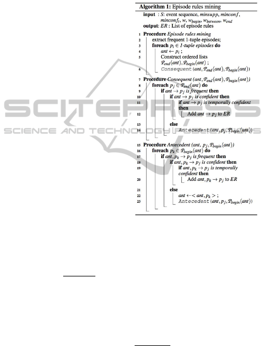
3.2 Steps of the Algorithm
We present now the different steps of our algorithm.
3.2.1 Initialization
Our algorithm starts by an initialization phase, which
reads the event sequence to extract all frequent events
and their associated occurrence timestamps. An event
represents a 1-tuple episode and will be denoted as
P. Table 1 presents the list of 1-tuple episodes of the
sequence S (Figure 1) and their associated occurrence
windows for minsupp = 2 (see Figure 3 line 2).
3.2.2 Prefix Identification
Episode rules are built iteratively by first fixing the
EpisodeRulesMiningAlgorithmforDistantEventPrediction
7

Table 1: 1-tuple episodes of S.
1-tuple episode p List of occurrence windows
A [1,1], [2,2], [7,7]
B [3,3], [8,8]
C [4,4], [9,9]
E [6,6], [10,10], [12,12]
F [6,6], [10,10], [12,12]
EF [6,6], [10,10], [12,12]
prefix (the first event of the antecedent). The an-
tecedent is denoted as ant. In the encoded sequence,
each 1-tuple episode p is viewed as a prefix of the
antecedent of an episode rule to be built. Once the
prefix of an episode rule R is fixed, its occurrence
windows OW(S,t
s
,t
e
) are known. For example, let
minsupp = 2, A can be considered as a prefix of an
episode rule. The list of occurrence windows of A =
([1,1],[2,2], [7,7]) (see Table 1).
3.2.3 Consequent Identification
A candidate consequent of an antecedent ant (here,
ant corresponds to a unique element, the prefix) is
chosen in the windows Win(S,t
s
,w) where: ant ⊆ I
t
s
.
Recall we want to form episode rules with a conse-
quent as far as possible from the antecedent. Thus, the
candidate consequents are not searched in the entire
window, they are searched only in Win
end
: where the
farthest candidates are. We construct P
end
(ant), the
ordered list of 1-tuple episodes that occur frequently
in Win
end
from Win(S,t
s
,w) that contains ant.
Let p
j
∈ P
end
(ant) be a candidate consequent of
ant. The episode rule R : ant → p
j
is formed and
its support is computed (see Figure 3 line 7). At this
stage, the occurrence windows of the episode rule R
are filtered to get minimal occurrences as well as to
preserve the anti-monotonicity property. This filter-
ing is done by counting only once the occurrence win-
dows containing the same occurrence of the conse-
quent p
j
. For example, let w
begin
= 2, w
end
= 2 and
w = 6. The episode rule R : A → E has three occur-
rence windows: ([1,6],[2,6],[7,12]). In the two first
occurrence windows, the consequent E is a common
1-tuple episode which occurs at timestamp t
6
. There-
fore, we consider only the interval [2, 6]. However, all
occurrencewindowsare kept in memory, to be used to
complete the antecedent. This enables not losing any
of the interesting episode rules which could be missed
if we kept only the minimal occurrences in memory.
Next, we compute the support of the correspond-
ing episode rules (see Figure 3 line 7).
We define the support of a rule P → Q, referred
to as supp
end
(P.Q), as the number of minimal occur-
rence windows computed above. It is different from
the traditional supp(P.Q) as it considers only occur-
rence windows where P occurs in Win
begin
and Q oc-
curs in Win
end
.
If R : ant → p
j
is not frequent, we consider that
p
j
cannot be a consequent of ant. This iteration is
stopped and the rule is discarded. There is no need to
complete the antecedent of the rule R, as whatever the
events that complete the antecedent are, the resulting
rule will not be frequent. The algorithm will iterate
on another consequent. If R : ant → p
j
is frequent, its
confidence is computed. its confidence is computed.
We define the confidence of a rule P → Q (see
Equation (1)) as the probability that the consequent
occurs in Win
end
, given that P appears in Win
begin
.
conf(P → Q) =
supp
end
(P.Q)
supp(P)
(1)
If the rule R : ant → p
j
is confident, this rule is
added to the set of rules formed by the algorithm.
It is minimal and has a consequent far from the an-
tecedent; it fulfills our goal. If the rule is frequent but
not confident, the antecedent of the rule R : ant → p
j
is completed (as in the next subsection).
For example, let w = 6, w
begin
= 2 and w
end
= 2.
For the episode rule R with prefix A. P
end
(A) =
[E,F,EF,A]. We first try to construct the episode
R with the consequent E. Thus, for R : A →
E, supp(R) = 2 and conf(R) = 2/3 = 0.67. For
minsupp = 2 and minconf = 0.7, R is frequent but
not confident, so its antecedent has to be completed.
3.2.4 Antecedent Completion
In this step, the antecedent, referred to as ant, is iter-
atively completed with 1-tuple episodes, placed on its
right side in the limit of the predefined sub-window
Win
begin
. At the first iteration: ant is a unique ele-
ment (the prefix) (see Figure 3 line 15). Recall that
we aim at forming rules having the last event of the
antecedent as far as possible from the consequent, so
as close as possible of the prefix. Thus, we construct
P
begin
(ant), the ordered list of 1-tuple episodes that
occur frequently after ant in the windows that starts
with it: the 1-tuple episodes that occur in Win
begin
.
Similarly to the consequent identification step, the
occurrence windows of the episode rule R are fil-
tered to get minimal occurrences and to preserve the
anti-monotonicity property. In addition, we apply the
same support, confidence verifications as for the con-
sequent identification.
To speed up the episode rules mining process we
use a heuristic. We propose to order the list of candi-
dates P
begin
(ant) in descending order of the number of
Win
begin
in which the candidates appear. We assume
that this number is highly correlated with the support
KDIR2014-InternationalConferenceonKnowledgeDiscoveryandInformationRetrieval
8

of the corresponding episode rules. So, in the traver-
sal of this list, when we observe that candidates tend
to form infrequent episode rules (several consecutive
1-tuple episodes lead to infrequent episode rules), we
stop the traversal. We consider that the remaining
candidates in this list will lead to infrequent episode
rules. This heuristic is used to reduce the number of
iterations. Although this heuristic may discard inter-
esting rules, it allows to reduce the iterations thus to
increase the size of the span of the rule (Win).
For example, let minsupp = 2 and mincon f = 0.7,
for R : A → E, P
begin
(A) = [B,C,A]. The antecedent of
R is completed with B and forms the episode rule R :
A,B → E. Thus, supp(R) = 2 and con f(R) = 2/2 =
1. The episode rule R is now confident, the phase of
completing its antecedent is stopped.
3.3 Temporal Confidence
Win
between
has been introduced so as to guarantee that
the consequent of an episode rule occurs in Win
end
,
after a w
begin
+ w
between
temporal distance from the
prefix of the episode rule. However, given an occur-
rence of the antecedent, the consequent may also oc-
cur closer to the antecedent, in the windowWin
between
,
which should affect the confidence of the rule. This
information may be important in some applications.
In the example of social networks, the prediction of a
negative event allows the company to act so as to pre-
vent its occurrence. So, it is important to mine rules
with a consequent that never occurs in Win
between
.
Indeed, predicting a consequent at a given distance,
which may appear closer is useless, even danger-
ous. Consequently, we have to take into consideration
the occurrence of the consequent in Win
between
. We
introduce a new measure, the temporal confidence,
which represents the probability that the consequent
occurs in Win
end
and only in it. For an episode rule
R : P → Q, this measure takes into account the sup-
port of P.Q when Q occurs only in Win
end
(and not in
Win
between
), denoted as supp
end
(P.Q). The temporal
confidence is defined as follows:
conf
t
(P → Q) =
supp
end
(P.Q)
supp(P.Q)
(2)
conf
t
(R) = 1 if for each occurrence of the consequent
of R in Win
end
, no occurrence of the consequent is
found in Win
between
. The temporal confidence of rules
from the previous section is computed and the rules
with a temporal confidence above minconf
t
are kept.
For example, let w = 6, w
begin
= 2 and w
end
= 2, the
temporal confidence of the frequent confident episode
rule R : A → E depends on the occurrences of E in
Win
between
which is equal to 1 (E appears in the times-
tamp t
10
in Win
between
). Thus, con f
t
(R : A → E) =
1/2 = 0.5. For minconf
t
= 0.5, R is temporally con-
fident and is a rule formed by our algorithm.
Figure 3: Episode rules mining algorithm.
4 EXPERIMENTAL RESULTS
In this section, we evaluate our algorithm through
the study of the characteristics of the episode rules
formed, as well as its performance in a prediction
task.
4.1 Dataset
The dataset we use is made up of 27,612 messages
extracted from blogs about finance. Messages are an-
notated using the Temis
1
software. Each message is
represented by its corresponding set of annotations
(items). For example, the message: “Not only my
1
http://www.temis.com
EpisodeRulesMiningAlgorithmforDistantEventPrediction
9

Table 2: 1-tuple episodes : length and support.
1-tuple episode
length (#items)
number(%)
support
min max mean median
1 498(76.4) 30 797 149.7 89.5
2
147(22,5) 30 376 71.5 55
3
7(1) 32 54 44.4 46
bank propose the best, but also online banks, so how
to optimize my savings? accounts in other banks? life
insurance? i need more info.” is annotated with the
following items : {(online banks, negative), (savings,
neutral), (life insurance, neutral ), (needs, neutral)} ,
where each item is associated with an opinion degree.
In this dataset, messages are annotated with 4.8
items on average, ranging from 1 to 50 and the me-
dian is 4. There are about 4,000 distinct annotations
(items), with an average frequency of 88.5. 1,981 of
these items have a frequency equal to 1. These items
will be automatically filtered out in the initialization
phase of our algorithm.
4.2 Characteristics of the Resulting
Rules
4.2.1 Initialization Phase
In this phase, frequent 1-tuple episodes are extracted
(1-tuple episode is made up of one or more items).
We fix minsupp for these 1-tuple episodes to 30. This
phase results in 652 frequent 1-tuple episodes. Ta-
ble 2 shows that the 1-tuple episodes are made up of
one to three items only. 1-tuple episodes are mainly
made up of one item (76% of them), which also have
a high support (on average 149.7).
In order to study the episode rules formed, we
make vary minsupp, minconf and w
between
one at a
time, while fixing others.
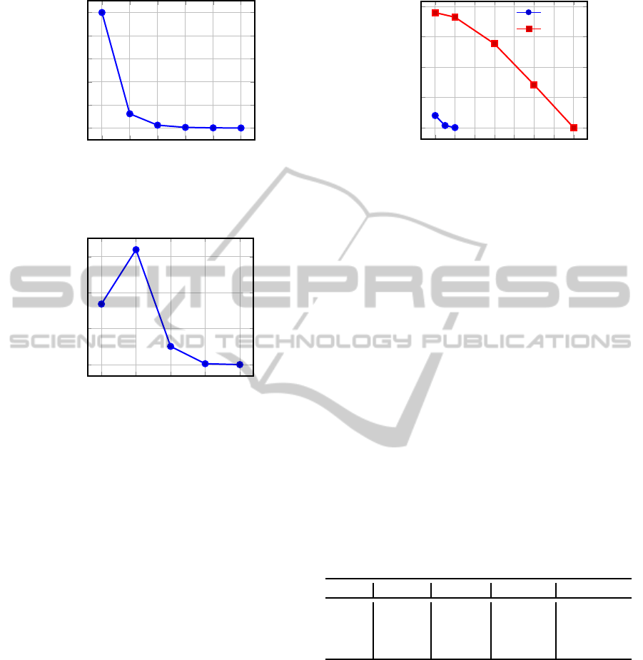
4.2.2 Making Vary minsupp
In Figure 4, we make vary minsupp from 10 to 35
to study the number of rules. Other parameters re-
main fixed: minconf = 0.4, w = 40 (with w
begin
=
20, w
between
= 10 and w
end
= 10). As expected, the
smaller minsupp, the higher the number of rules.
When minsupp is fixed to 10, the number of rules
is high (about 10
4
). Recall that the number of 1-
tuple episodes is only 652. However, the number
of rules is dramatically decreased when minsupp is
increased: only 1,200 when minsupp = 15 and 250
when minsupp = 20. These low values are due to the
small average frequency of 1-tuple episodes (about
88). In addition, these rules represent a temporal de-
pendence between the antecedent and the consequent
which, in these experiments, is at least w
between
= 10.
This may explain the low number of rules. A thor-
ough study shows that their average confidence in-
creases with minsupp.
4.2.3 Making Vary minconf
We make vary minconf from 0.1 to 0.5. Figure 5
presents the number of episode rules according to the
value of minconf (minsupp = 20, w = 40 (w
begin
=
20, w
between
= 10 and w
end
= 10)). The number of
rules is particularly high with minconf = 0.2. This is
explained by the way our rules are formed. When the
confidence of a rule does not exceed mincon f, its an-
tecedent is extended. Given an antecedent ant, events
in P
begin
(ant) (up to 652) are appended to it, resulting
in a large number of candidate rules. Some of them
are confident, which explains the increase of the num-
ber of rules. When minconf exceeds 0.2, the number
of rules decreases.
Table 3 presents the length of the antecedent of
the rules (in number of events), according to minconf.
The maximum length of an antecedent is three. Thus,
our algorithm, forms rules with a small antecedent,
which was one of its goals. The average length of the
antecedent increases with minconf: when minconf =
0.1, most of the rules have an antecedent of length
1, whereas when minconf = 0.3, most of the rules
have an antecedent of length 2. This was expected,
as minimal antecedents are searched. Indeed, when a
frequent rule has a confidence below minconf, its an-
tecedent is extended,till it is confidentor not frequent.
So, the higher minconf, the larger the antecedents. A
thorough study shows that the average length of oc-
currence windows of the antecedents is 8 timestamps
(for antecedents of length 2 and 3), which is smaller
than the span of the antecedent (w
begin
). We conclude
that our algorithm succeeds in forming rules with a
distant consequent, a small antecedent (in length and
time) and a relatively high confidence.
Table 3: Antecedent length when making vary minconf .
minconf #Rules
%Rules
ant 1 ant 2 ant 3
0.1 16,850 57.2 42.84 0
0.2
31,972 4.2 95.6 0.2
0.3
5,072 0.9 97.5 1.6
0.4
251 0.8 90.9 8.3
0.5
9 0 100 0
4.2.4 Making Vary w
between
We now focus on the number of rules formed, accord-
ing to w
between
(w and w
begin
remain fixed), presented
KDIR2014-InternationalConferenceonKnowledgeDiscoveryandInformationRetrieval
10

10
15
20
25
30
35
0
0.2
0.4
0.6
0.8
1
·10
4
minsupp
#Rules
Figure 4: number of rules (10
4
) vs. minsupp.
0.1 0.2 0.3 0.4
0.5
0
1
2
3
·10
4
mincon f
#Rules
Figure 5: number of rules (10
4
) vs. minconf.
in Figure 6 where minsupp = 20 and minconf = 0.4.
Two values of w are studied: w = 40 (with w
begin
=
20) and w = 100 (w
begin
= 20). Notice that the cases
w
between
= 0 represent similar cases than state of the
art. We note that the larger w
between
, the smaller the
number of rules. Two reasons may explain this de-
crease. First, when w
between
increases, w
end
(the win-
dow in which the consequent is searched) decreases,
as well as the number of consequents studied. Sec-
ond, the larger w
between
, the more distant the conse-
quent, thus the lower the probability of having a de-
pendence between the antecedent and the consequent.
However, even with a large value of w
between
, some
rules are formed: 210 rules when w
between
= 70. We
conclude that there is actually a temporal dependence
between messages in blogs. When the minimal dis-
tance between the antecedent and the consequence is
50, more than 140k confident rules are formed: there
is a strong dependence between messages with such
a distance. For example, when w = 100 an episode
rule: (price, positive), (information, positive) → (buy,
positive), means that when someone talks about the
price of an article then asks for information, he/she
will buy this article after some time. Thus, we have
time to recommend him similar articles or to propose
to him a credit to buy it.
0 10 20 30 40
50 60
70
0
1
2
3
4
·10
5
w
between
#Rules
w = 40
w = 100
Figure 6: number of rules (10
5
) vs. w
between
.
Influence of minconf
t
: In this section we study
the temporal confidence of the resulting rules. Table 4
presents the evolution of the temporal confidence ac-
cording to w
between
. We remark that the smaller
w
between
, the higher the temporal confidence: the con-
sequent does rarely occur between the antecedent and
the consequent when the gap between them is small,
which was expected. When w
between
= 30, the aver-
age temporal confidence is 0.6, which is quite high. A
thorough study shows that among 2.7· 10
5
rules (see
Figure 6), about 40 ones have a temporal confidence
equal to 1 (the consequent never occurs in Win
between
)
and 1,400 rules have a temporal confidence higher
than 0.9 (the consequent appears in Win
between
in less
than 10% of the cases). This shows that in this dataset
there is a strongtemporal dependencebetween events,
and that some events are interdependent at a distance
of 30.
So, when exploiting the temporal confidence as a
filter, a great number of rules remain.
Table 4: w
between
vs. Temporal confidence (conf
t
).
w
between
min-conf
t
max-conf
t
mean-conf
t
median-conf
t
70 0 0.5 0.2 0.2
50
0.2 0.9 0.4 0.4
30
0.3 1 0.6 0.6
10
0.2 1 0.9 0.9
4.3 Performance
In this section we focus on the accuracy of the rules
formed when they are used to predict events, and we
perform a comparison of the rules with those of a tra-
ditional algorithm.
We evaluate the accuracy of our algorithm with
the traditional recall and precision measures. The
episode rules are trained on the first 75% messages
and are tested on the 25% of messages left. Fig-
ure 7 presents the resulting precision and recall at
20. We fix minsupp = 20, minconf = 0.4, w = 100
EpisodeRulesMiningAlgorithmforDistantEventPrediction
11

and w
begin
= 20. We make vary w
between
from 10 to
70. First of all, mention that two precision and re-
call values with two different values of w
between
are
not directly comparable as they are not computed on
the same data (the windows Win
end
, on which they
are computed vary in size). Both precision and re-
call curves decrease as w
between
increases. This was
expected as the number of rules decreases. When
w
between
= 70 (and w
end
= 10), both precision and re-
call values are quite low. This was expected as the
rules aim at predicting events distant to at least 70, in
an occurrence window of length w
end
=10. The prior
probability of predicting events accurately is low. Let
us now consider w
between
= 30, as in the previous sec-
tion. We can see that both precision and recall values
are quite high. When an event is predicted, in 37% of
the cases, it actually occurs and events that occur in
the sequence are predicted by our rules in 70% of the
cases.
10 20 30 40
50 60
70
0
0.2
0.4
0.6
0.8
w
between
precision-recall
precision@20
recall@20
Figure 7: precision, recall vs. w
between
.
Comparison with Minepi: Contrary to tradi-
tional algorithms, our algorithm forces a minimum
gap of length w
between
between the antecedent and the
consequent of an episode rule. Our algorithm can be
comparedto traditional algorithms when w
between
= 0.
Since we apply the minimal occurrence-based fre-
quency, we choose to compare it to the well-known
Minepi (Mannila et al., 1997). For minsupp = 20,
minconf = 0.4, w = 40, Minepi forms more than
136, 000 episode rules, whereas our algorithm (when
w
between
= 0) extracts about 40,000 episode rules
(70% less). This decrease is due to two reasons. First,
the constraint about the position of consequent of the
episode rules from our algorithm (in this case the dis-
tance between the antecedent and the consequent is
at least 20, even if w
between
= 0), makes the num-
ber of rules resulting from our algorithm lower (also
their support is lower). Second, our algorithm aims
at forming minimal rules, thus few rules with a large
antecedent are formed. We remark that 25% of the
rules extracted by Minepi have an antecedent larger
or equal to 3, whereas this rate is only 1.8% for our
algorithm.
Here an example of an episode rule extracted by
both our algorithm (w
between
= 0) and by Minepi:
(credit, positive), (consultant, positive) → (loan sub-
scription, positive).
Here is a rule that has not been extracted by our
algorithm, as it does not satisfy the desired character-
istics of episode rule (minimal antecedent): (consul-
tant, neutral), (interest rate, positive) → (request in-
terest rate 0, positive), where the antecedent occurs in
5 timetstamps and consequent occurs in the 7
th
times-
tamp. This rule is useful in traditional cases of event
prediction (prediction of close events). However, it
does not fit our objective of early prediction of dis-
tant events, as the antecedent is so long both in time
and in number and the consequent is too close to the
antecedent.
Concerning the running time, our algorithm runs
5 times faster than Minepi when w = 100, and 4 times
faster when w = 40. This decrease is due to two fac-
tors. The first one is related to the consequent, which
is fixed at an early stage of the algorithm and which
allows to filter infrequent rules early in the process.
The second one is due to the fact that our algorithm
mines rules with a minimal antecedent, which avoids
some iterations once a confident rule is found.
5 CONCLUSION
In this paper, we propose an algorithm that mines
episode rules, in order to predict distant events. To
achieve our goal, the algorithm mines serial episode
rules with distant consequent. We determine several
characteristics of the episode rules formed: minimal
antecedent, and a consequent temporally distant from
the antecedent. A new confidence measure, the tem-
poral confidence, is proposed to evaluate the confi-
dence on distant consequents. Our algorithm is eval-
uated on an event sequence of annotated social net-
works messages. We show that our algorithm is effi-
cient in extracting episode rules with the desired char-
acteristics and in predicting distant events.
Since we use data from social networks, we aim to
use multi-thread sequences. This means that we con-
struct a sequence for each thread of messages: user
messages thread, topic messages thread and discus-
sion thread, etc. and the algorithm is run on each one.
Using multi-threadsequences allows to build more di-
verse episode rules which are all together more sig-
nificant. The presence of a rule in several threads will
increase its confidence.
KDIR2014-InternationalConferenceonKnowledgeDiscoveryandInformationRetrieval
12

ACKNOWLEDGEMENTS
This research is supported by Cr´edit Agricole S.A.
REFERENCES
Achar, A., Sastry, P., et al. (2013). Pattern-growth based
frequent serial episode discovery. Data & Knowledge
Engineering, 87:91–108.
Agrawal, R., Imieli´nski, T., and Swami, A. (1993). Min-
ing association rules between sets of items in large
databases. In ACM SIGMOD Record, volume 22,
pages 207–216. ACM.
Cho, C.-W., Wu, Y.-H., Yen, S.-J., Zheng, Y., and Chen,
A. L. (2011). On-line rule matching for event predic-
tion. The VLDB Journal, 20(3):303–334.
Gan, M. and Dai, H. (2011). Fast mining of non-derivable
episode rules in complex sequences. In Modeling De-
cision for Artificial Intelligence. Springer.
Huang, K.-Y. and Chang, C.-H. (2008). Efficient mining of
frequent episodes from complex sequences. Informa-
tion Systems, 33(1):96–114.
Laxman, S., Sastry, P., and Unnikrishnan, K. (2007). A
fast algorithm for finding frequent episodes in event
streams. In 13th ACM SIGKDD. ACM.
Laxman, S. and Sastry, P. S. (2006). A survey of temporal
data mining. Sadhana, 31(2).
Luo, J. and Bridges, S. M. (2000). Mining fuzzy associa-
tion rules and fuzzy frequency episodes for intrusion
detection. Int. J. of Intelligent Systems, 15(8):687–
703.
Mannila, H., Toivonen, H., and Verkamo, A. I. (1997). Dis-
covery of frequent episodes in event sequences. Data
Mining and Knowl. Discovery, 1(3):259–289.
M´eger, N. and Rigotti, C. (2004). Constraint-based mining
of episode rules and optimal window sizes. In PKDD
2004, pages 313–324. Springer.
Neeraj, S. and Swati, L. S. (2012). Overview of non-
redundant association rule mining. Research Journal
of Recent Sciences ISSN, 2277:2502.
Ng, A. and Fu, A. W.-C. (2003). Mining frequent episodes
for relating financial events and stock trends. In Ad-
vances in Knowledge Discovery and Data Mining,
pages 27–39. Springer.
Pasquier, N., Bastide, Y., Taouil, R., and Lakhal, L. (1999).
Discovering frequent closed itemsets for association
rules. In Database Theory-ICDT, pages 398–416.
Springer.
Rahal, I., Ren, D., Wu, W., and Perrizo, W. (2004). Mining
confident minimal rules with fixed-consequents. In
16th IEEE ICTAI 2004.
EpisodeRulesMiningAlgorithmforDistantEventPrediction
13