Linearizing Controller for Higher-degree Nonlinear Processes with

Compensation for Modeling Inaccuracies

Practical Validation and Future Developments

Pawel Nowak

, Jacek Czeczot

, Tomasz Klopot

, Mateusz Szymura

and Bogdan Gabrys

Silesian University of Technology, Faculty of Automatic Control, Electronics and Computer Science

Institute of Automatic Control, Gliwice, Poland

Smart Technologies Research Centre, Computational Intelligence Research Group, Bournemouth University,

Fern barrow, Poole, BH12 5BB, U.K.

Keywords: Adaptive Control, Soft Sensors, Linearizing Control, Practical Validation.

Abstract: This work shows the results of the practical implementation of the linearizing controller for the example

laboratory pneumatic process of the third relative degree. Controller design is based on the Lie algebra

framework but in contrast to the previous attempts, the on-line model update method is suggested to ensure

offset-free control. The paper details the proposed concept and reports the experiences from the practical

implementation of the suggested controller. The superiority of the proposed approach over the conventional

PI controller is demonstrated by experimental results. Based on the experiences and the validation results,

the possibilities of the potential application of the data-driven soft sensors for further improvement of the

control performance are discussed.

1 INTRODUCTION

The application of the linearizing technique for the

control of the higher relative degree nonlinear

processes was extensively studied as a very

promising approach, which provides the general

framework for compensating for the complex

dynamics of the nonlinear processes (Isidori, 1989;

Henson and Seborg, 1997). In summary, this

concept allows for deriving the nonlinear control law

based on the nonlinear model of a process

transformed using the Lie algebra. After assuming

the reference model of the corresponding order, the

final form of the controller is derived, which

compensates for the process nonlinearities and

allows for cancellation of the process higher degree.

The results of the application of this technique to

the control of the processes of the higher relative

degree were reported in a relatively large number of

publications but all of them were based on the

simulation studies. The exceptions are the cases, in

which the linearizing control technique is based on

the simplified first-order dynamical model of a

process - the higher relative degree is compensated

by the proper conservative tuning while the offset-

free control is ensured by the compensation for the

modeling inaccuracies by the application of the

integral action (Lee and Sillivan, 1988; Metzger,

2001) or by the on-line model update (Rhinehart and

Riggs, 1991; Czeczot, 2001).

It must be said that, even if the dynamics of the

real processes usually is of higher relative degree,

the idea of the linearizing technique accounting for

such degree is not popular in the industrial control

applications, due to the following difficulties:

 it requires complex mathematical calculations

based on the nonlinear model of a process;

 offset-free control is possible only if the

model of a process is perfect;

 computational complexity of the linearizing

controller is relatively high.

Another important difficulty that must be faced

when the linearizing control technique is to be

applied in practice is that the measurement data from

the disturbances and from the process state variables

are required. Generally, when the appropriate

sensors are not accessible, these quantities must be

estimated by implementing observers based on the

process model (Albertos and Goowin, 2002;

Kravaris et al., 2013) or by applying suitable data-

driven soft sensors (Fortuna et al., 2007; Lin et al.,

691

Nowak P., Czeczot J., Klopot T., Szymura M. and Gabrys B..

Linearizing Controller for Higher-degree Nonlinear Processes with Compensation for Modeling Inaccuracies - Practical Validation and Future

Developments.

DOI: 10.5220/0005048606910698

In Proceedings of the 11th International Conference on Informatics in Control, Automation and Robotics (ICINCO-2014), pages 691-698

ISBN: 978-989-758-039-0

 2014 SCITEPRESS (Science and Technology Publications, Lda.)

2007; Kadlec et. al 2009). The hybrid approach for

this problem is also possible.

Finally, for the control of the processes of the

higher relative degree r > 1, the difficulties in

controller tuning can be expected. Generally, for

such a case, at least r tuning parameters must be

adjusted and there are no simple methods that can be

easily applied in practice. At the same time, it should

be noticed that the linearizing controller requires the

feedback from higher order time derivatives of the

controlled variable to compensate for the process

dynamics. These r-1 consecutive derivatives must be

computed based on the noisy measurement data.

In this work it is shown how the general

linearizing technique can be applied for the

improved control of the pneumatic process of the

third relative degree. The method for on-line

compensation for modeling inaccuracies is also

suggested that ensures offset-free control. The

experiences and results from the stage of practical

implementation and validation are reported and

discussed. Finally, based on these experiences and

validation results, the potential options for further

improvements are discussed and suggested,

concentrating on the possibilities of the application

of data-driven soft sensors derived from a family of

statistical, computational intelligence and machine

learning approches.

2 CONTROLLER DESIGN

In this paper, the model-based linearizing control of

the nonlinear processes of the higher relative degree

r > 1 is considered. It is assumed that the process is

described by the following standard nonlinear state

equations derived from first principle modelling

where functions F(.) and h(.) are known while x and

d respectively denote the process states and

disturbances:















xhY

udxF

(1)

The control goal is to stabilize the controlled output

Y at the set point Y

by manipulating the input u.

For the model-based linearizing controller

synthesis, after applying Lie algebra (e.g., Isidori,

1989; Henson and Seborg, 1997), the model (1)

should be rearranged into the known part of the

dynamical equation of the r-th order, describing

directly the controlled variable Y:



RudxYHdxYH





partknown

,,,,

(2)

Due to modelling inaccuracies, any controller

based only on the known part of Eq. (2) cannot

ensure offset-free control without additional

application of the integration of the regulation error

or without any other on-line compensation for

modelling error. Thus, based on the idea of the

Balance-Based Adaptive Control (B-BAC) (e.g.

Czeczot, 2001, 2006) or more generally on the

additive disturbance estimate for Model Predictive

Control (MPC) (e.g. Maciejowski, 2002), the single

additive parameter R

completes the known part of

Eq. (2). R

accounts for modelling inaccuracies

which can be easily and effectively compensated by

on-line estimation of its value.

For the controller design, the r-th order reference

model can be assumed for the closed loop dynamics:











ksp



(3)

with

.. λ

r-1

denoting the tuning parameters and

then, after substituting

by its on-line estimate

and inversing, the adaptive linearized controller for

the considered process can be derived as:



sp k Y

YY HYxdR

HYxd







  





(4)

The controller (4) potentially is able to

compensate for the process nonlinearities and its

higher order dynamics. It must be implemented

jointly with the estimation procedure for computing

the value of

and only then it can ensure the

offset-free control. For this purpose, a simple

method can be suggested taking advantage of the B-

BAC methodology (Czeczot, 1998; Stebel

et al.,

2014), using the discretized model (2) and the

measurement data for

Y, x and d. After discretization

of Eq. (2), the following equation can be derived:









,1,2,

rr r

RYi T R i ii i

RYi i

TR Y T H H u





    

 



(5)

where

i denotes the i-th sampling, T

is the

discretization instant,





represents the r-th

order finite backward difference operator and





dxYHH ,,

1,1







dxYHH ,,

2,2



. Due to the

ICINCO2014-11thInternationalConferenceonInformaticsinControl,AutomationandRobotics

692

presence of the measurement noise represented by

the additive error

ε, Eq. (5) is not recommended for

directly calculating the estimate

and thus the

estimation procedure based on the WRLS (Weighted

Recursive Least-Squares) method is applied to

minimize the influence of this noise on the

estimation accuracy. Eq. (5) defines the measurable

auxiliary variable

w and it has the form of the linear

equation affine to the unknown parameter

with

the constant regressor (

–T

). Consequently, it allows

for the application of the simplified scalar discrete-

time form of the WRLS equations where

α(0,1)

denotes the forgetting factor:









(6a)





1,1,,

ˆˆˆ





Rii

RiYiY

RTwPTRR ,

(6b)

with the initial values:

> 0 and freely but

reasonably chosen

. The dynamical properties

of the estimation procedure (6) are equivalent to the

estimation procedure suggested previously for the

B-BAController in the form dedicated for the

processes of the unitary relative degree (Czeczot,

2006a; Klopot, Czeczot and Klopot, 2012; Stebel et

al., 2014). The accurate estimation is ensured

without necessity of applying any additional

excitation input signals. In fact, even at the steady

state, the estimate

always converges to its true

value R

with the rate of convergence depending

only on the value of the forgetting factor α. For the

considered case, the significant difference is that the

estimation is based on the higher order dynamical

model and thus the on-line calculation of the

backward finite differences





in Eq. (5) is

required, based on the noisy measurements.

When the controller (4) with the estimation

procedure (6) are to be applied in practice, there are

some difficulties that must be dealt with:

 the higher relative degree r > 1 requires

computing higher order time derivatives, both

for the controller (4) and for the estimation

procedure (6) - for this purpose, the backward

finite differences of the respective order can

be applied but then the calculations would be

based on the noisy measurement data of Y;

 tuning requires adjusting r parameters λ

.. λ

r-1

for the controller (4) and the forgetting factor

α for the estimation procedure (6);

 the measurement data for the states x and for

the disturbances d are required; the not

measurable ones should be computed by

applying an observer designed based on the

model (1) (Albertos and Goodwin, 2002;

Kravaris et al., 2013) or as data-driven soft

sensor (Kadlec and Gabrys, 2008; 2009;

Kadlec et al., 2009).

Summarizing, the suggested approach is very

promising and it ensures very good control

performance during the simulation experiments in

the application to a various higher-degree nonlinear

processes. At the same time, from the practical

viewpoint, it requires relatively high computational

effort and it is potentially sensitive to the

measurement noise. Thus, the aim of this paper is to

verify in practice if the application of the controller

(4) with the estimation procedure (6) can improve

the control performance that would be worth such

additional modelling and implementation effort.

3 PRACTICAL VALIDATION

In the paper, the experimental setup of three serially

connected pneumatic tanks presented in Fig. 1 is

considered as the example process to be controlled.

The respective volumes of the tanks are V

= 5 [L],

= 2 [L] and V

= 0.75 [L] and the corresponding

relative pressures at each tank are denoted as p

, p

[bar]. The respective pressure capacities are

denoted as c

, c

and c

[m*s

]. The system is

manipulated by the supplying air pressure p

[bar]

and the air flows between the tanks through the

constant pneumatic resistances R

, R

[m*s]. In

the last tank, the air flows out through the adjustable

pneumatic resistance R

[m*s] and the relative

pressure outside the tank is denoted as p

[bar]. The

supplying relative pressure p

is adjustable by the

proportional valve MPPES-3-1 from Festo within

the range 0 - 4 [bar]. All the pressures p

, p

are measured on-line by the SDE1 pressure sensors

and the pneumatic resistance R

at the outlet from

the third tank can be changed by automatic

switching between two pneumatic valves of different

resistance. The relative pressure p

= 0. The

pneumatic process is connected to the SCADA

system (Golda, 2013) written in zenon from COPA-

DATA and the on-off valves are controlled by the

controller CPX-CEC-C1 from Festo.

LinearizingControllerforHigher-degreeNonlinearProcesseswithCompensationforModelingInaccuracies-Practical

ValidationandFutureDevelopments

693

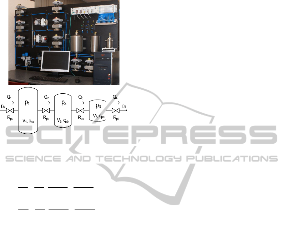
Figure 1: Pneumatic experimental setup.

For the controller synthesis, the mathematical

model of the process has been derived in the form of

Eqs. (1), assuming laminar flow (Golda, 2013):





























































43323

212

cdt

pdpcpc

pcpbpb

pbpa

(7)

For the chosen operating point, the values of the

model parameters have been identified off-line from

the measurement data as: c

= 6*10

-8

, c

= 2.5*10

-8

= 1*10

-8

, R

= 0.25*10

, R

= 0.6*10

= 12*10

and R

= 25 *10

. Readers should note

that this linear flow modelling is a simplification

because for some operating regions, the flow in the

real process is nonlinear.

The control goal is defined to stabilize the

pressure Y = p

at the set point Y

by manipulating

the supplying pressure u = p

. The process is

disturbed by the relative pressure p

and by the

outlet pneumatic resistance R

. Its relative degree is

r = 3 and assuming constant disturbances, the model

(7) can be rearranged into the dynamic equation of

the form of Eq. (2), describing the dynamics of the

controlled variable:

 

Ypdpd

pdpds

RpREYRD

pRCpRBAp





(8)

where the expressions for A, B(R

), C(R

), D(R

E(R

) are given in the Appendix. After defining:



















211

pRE

YRDpRCpRBH

pdpdpd











(9a)







(9b)

the form of the controller (4) can be directly applied,

jointly with the estimation procedure (6) for the

unknown parameter

. Assuming p

= 0, this

approach requires the measurement data from the

disturbance

and from the other states p

, p

Additionally, based on the measurement data, 1

, 2

and 3

order time derivatives of the controlled

pressure

Y = p

must be computed numerically.

During practical implementation and validation,

it was assumed that only the relative pressures

u = p

and

Y = p

are measurable on-line. Additionally, the

values of the disturbing R

for the considered

operating points were approximately identified off-

line from measurement data so they could be

assumed to be known. The moments of the

switching between different values of the disturbing

resistance

were known as well.

The suggested controller (4) requires the

measurement data from the relative pressures

, p

which are assumed to be not measurable. Thus, it

was decided to apply the model (7) excited by the

same signals as the real process as the open-loop

observer, to avoid the additional dynamics

introduced by the correction term required for on-

line update of the closed-loop observer. This

approach is justified by the fact that in practice,

when the model is incorrect, the correction term

does not ensure perfect state estimation and this

inaccuracy must be compensated anyway. For the

suggested approach, the estimation procedure

ensures the compensation of any modelling

inaccuracies directly in the control law so the

inaccuracy of the observer is acceptable and there is

no need to introduce the additional dynamics

resulting from the its correction term that yet has to

be tuned.

The first attempt to the practical implementation

was based on the numerical computation of the 1

and 3

order time derivatives of the controlled

pressure

Y = p

directly from the measurement data

by successive application of the library functions

DERIVATIVE accessible in the programming

environment CoDeSYS. The results were



ICINCO2014-11thInternationalConferenceonInformaticsinControl,AutomationandRobotics

694

unacceptable because all the pressures are measured

by the sensors equipped with A/D converters of

limited resolution which results in significant and

unpredictable quantization effect that can be

considered as a type of measurement noise.

Consequently, the consecutive time derivatives

computed based on this data vary in a wide range

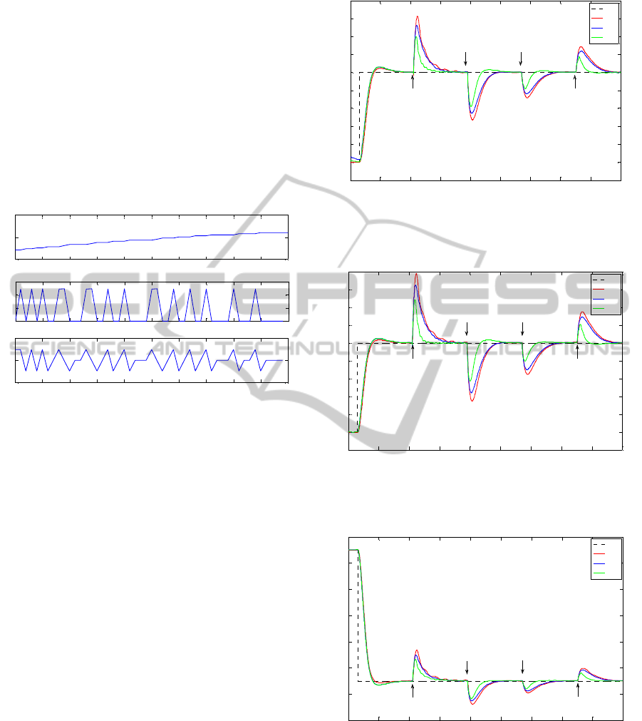
producing peaks, which is presented in Fig. 2. The

higher order derivatives are corrupted even more and

more significantly and these peaks result in very

large chattering of the manipulated variable

computed by the controller (4), which is

unacceptable.

Figure 2: Example magnified results for computing the 1

(second diagram) and 2

(third diagram) time derivatives

of the controlled variable from measurement data of the

original signal (first diagram).

Because the model (7) must be integrated

numerically jointly with the controller (4) and the

estimation procedure (6) (as the open-loop observer)

to provide the required information about the

pressures

, p

, it was decided to substitute the

measurement data of the controlled pressure

by its

value reconstructed by the model (7) for computing

the consecutive time derivatives. This approach

allows to avoid the quantization effect because the

variations of the modeled pressure

are smooth.

Consequently, unacceptable chattering in the

manipulated variable disappears and the control

performance of the suggested linearizing controller

is acceptable from the practical viewpoint.

Figures 3 - 5 show the comparative experimental

results for three different operating points defined by

the corresponding set point

. Each experiment

was carried out under the same scenario including

the initial step change of the set point and the

successive step changes of the disturbing resistance

applied to the system and shown in all Figures.

Figure 3: Experimental results of the control performance

for the operating point Y

= 1.

Figure 4: Experimental results of the control performance

for the operating point Y

= 1.5.

Figure 5: Experimental results of the control performance

for the operating point Y

= 0.5.

During experiments, the conventional PI

controller was applied as a benchmark, due to its

huge popularity among industrial engineers (it is still

the most frequently used control algorithm in the

existing industrial control loops), even if the

25 25.5 26 26.5 27 27.5 28 28.5 29 29.5 30

0.95

1.05

Y = p

[bar]

25 25.5 26 26.5 27 27.5 28 28.5 29 29.5 30

0.01

0.02

0.03

dY/dt

25 25.5 26 26.5 27 27.5 28 28.5 29 29.5 30

-0.5

0.5

time

[

]

Y/dt

0 50 100 150 200 250 300 350 400 450

0.4

0.5

0.6

0.7

0.8

0.9

1.1

1.2

1.3

1.4

time [s]

Controlled variable Y = p

[bar]

Control performance

Lin

Linff

t = 105s

Rpd 25 -> 300

t = 285s

Rpd 25 -> 16

t = 195s

Rpd 300 -> 25

t = 375s

Rpd 16 -> 25

0 50 100 150 200 250 300 350 400 450

0.9

1.1

1.2

1.3

1.4

1.5

1.6

1.7

1.8

1.9

time [s]

Controlled variable Y = p

[bar]

Control performance

Lin

Linff

t = 195s

Rpd 300 -> 25

t = 285s

Rpd 25 -> 16

t = 375s

Rpd 16 -> 25

t = 105s

Rpd 25 -> 300

0 50 100 150 200 250 300 350 400 450

0.2

0.4

0.6

0.8

1.2

1.4

1.6

time [s]

Controlled variable Y = p

[bar]

Control performance

Lin

Linff

t = 195s

Rpd 300 -> 25

t = 375s

Rpd 16 -> 25

t = 285s

Rpd 25 -> 16

t = 105s

Rpd 25 -> 300

LinearizingControllerforHigher-degreeNonlinearProcesseswithCompensationforModelingInaccuracies-Practical

ValidationandFutureDevelopments

695

methods for design of the PID-based control loops

are still developing,

e.g. (Åström and Hägglund,

2005; Ang, Chong and Li, 2005; Jin and Liu, 2014).

Initially,

PI controller was tuned for a single

operating point, using the Chien-Hrones-Reswick

tuning method.

Linff represents the suggested

controller with the feedforward action from the

varying value of

included in the function H

(.)

defined by Eq. (9a) and in the model (7) computed

jointly with the suggested controller.

Lin is the same

controller but without such action where the constant

value of

identified for the chosen operating point

is applied for the whole experiment. Initial tuning of

both

Linff and Lin controllers was based on locating

the roots of the characteristic polynomial

+λ

s+λ

as the negative real values to ensure

stable reference model (3) (Henson and Seborg,

1997). Finally, all controllers were retuned manually

to ensure the same tracking properties with possibly

small overregulation to ensure fair comparison

(

= 1.55, T

= 10.03 [s] for PI controller and

= λ

= 0.7, λ

= 0.08 for Linff and Lin controllers).

The forgetting factor for the estimation procedure

(6) was adjusted as

α = 0.95.

The results show the superiority of the suggested

controller. Even

Lin ensures smaller overregulations

for disturbance rejection in comparison with the

benchmark conventional

PI controller. The

application of Linff that incorporates the information

about the variations of the disturbing resistance

allows for more significant improvement in the

disturbance rejection by ensuring shorter settling

time and smaller overregulations, with the same

smooth tracking properties.

4 CONCLUSIONS

This paper reports the preliminary results of the

practical validation of the proposed control method

in the application to the example pneumatic process

of the relative degree

r = 3. After assuming the

closed loop reference model of the 3

order, the

linearizing controller is derived based on the

simplified first-principle model. Inclusion of the

higher order time derivatives of the controlled

pressure

Y = p

in the control law provides the

compensation for the higher relative degree of the

process dynamics. Potential modelling inaccuracies

in the steady state are compensated by the on-line

estimation of the additive parameter

, which

ensures the offset-free control. The simplified first-

principle model of the process must be also

numerically integrated on-line and applied as the

open loop observer to provide the required

information about not measurable states and to

enable computing the higher order time derivatives

of the controlled pressure, which is necessary due to

poor quality of the measurement data.

The experimental results show the practical

applicability of the suggested approach and its

superiority over the conventional

PI controller, even

in the case when there is no feedforward action from

the disturbing pneumatic resistance

. Inclusion of

this action additionally improves the control

performance even if the simplified first-principle

model of the process used both for the controller

synthesis and as the open loop observer is simplified

and partially inaccurate.

The practical disadvantage of the proposed

controller is its relatively high mathematical

complexity. It requires possibly accurate first-

principle model that then must be rearranged by

applying Lie algebra into the corresponding higher

order equation describing the dynamics of the

controlled variable. Even for the simplified process

model, the calculations are complex and they

become more complex if the highly nonlinear model

of the process is to be applied for this purpose.

5 FUTURE DEVELOPMENTS

In the considered case, the successful practical

implementation of the suggested adaptive linearizing

controller requires on-line numerical solving of the

simplified model (7) of the process to provide the

information about two not measurable state variables

, p

and about the controlled pressure p

that is

measurable but the quality of the measurement data

does not allow for computing the consecutive

required time derivatives.

The model (7) operates as the open-loop

observer and thus its accuracy is of the highest

importance. Especially it is important to ensure

possibly the best compensation for the higher degree

dynamics of the real process in the transients. The

results presented in this work were obtained for the

case when the model (7) is time invariant with the

only exception of the feedback from the

approximately known measurable disturbance

All modeling inaccuracies are compensated by the

on-line estimation of the additive parameter

but

in fact, this approach is fully effective only in the

steady state to ensure offset-free control. A surely

much better control performance could be obtained

if the model (7) was additionally adaptively updated

ICINCO2014-11thInternationalConferenceonInformaticsinControl,AutomationandRobotics

696

to ensure possibly highest modeling accuracy of the

process dynamics. For this purpose, a range of data

driven methods for designing the adaptive soft

sensors (Fortuna

et al., 2007; Lin et al., 2007;

Kadlec et. al, 2011) can be considered and combined

with the model (7).

As one of the key aspects of the proposed

method's success is either the availability of the

measurements or their robust estimation procedure

the data driven soft sensors could also be employed

in the case of individual measurements prediction

like in the case of values which are only infrequently

measured (e.g. pressure values

and p

from our

example) or for the smoothing/interpolation

purposes to avoid numerical problems resulting from

the usage of inaccurate hard sensors (e.g. controlled

pressure

in our example).

There have been great advancements made in the

learning algorithms used for the construction and

adaptation of soft sensors and their multitude of

applications and successful deployments have been

summarized in comprehensive reviews (Lin

et al.,

2007; Kadlec et. al, 2009; Kadlec et. al 2011) and

textbooks, e.g. (Fortuna

et al., 2007). The illustrated

ability to start working with only few historical

samples available (Kadlec and Gabrys, 2010) or to

adapt and provide robust prediction in dynamically

changing environments with noisy measurements

(Kadlec and Gabrys, 2008, 2009, 2011) make the

modern, intelligent soft sensing approaches a very

attractive proposition to combine with model-based

control approaches either as a replacement of the

traditional observers (which require the knowledge

of the plant model) or by providing information

about variables which cannot be measured or can be

measured only infrequently making them of limited

use for control purposes. Such variables can be

modeled and predicted on the basis of other

measurable process variables which soft sensor

techniques successfully exploit. Our future work will

therefore focus on enhancing and robust evaluation

of the proposed nonlinear model-based control

algorithms dedicated for the processes of the higher

relative degree, utilizing a variety of data driven soft

sensing approaches. One possibility is to substitute

the first-principle process model by the data-driven

soft sensor based on the initial off-line learning from

the measurement data and providing the prediction

of the required state and controlled variables. The

other approach could be based on the adaptive data-

driven update of the existing first-principle model to

ensure the on-line compensation for modeling

inaccuracies. In the latter, if the compensation was

accurate, it would be possible to remove the

estimation procedure for the additive parameter

from the final form of the controller that now

ensures the offset-free control in the presence of the

steady state modeling inaccuracy.

The results presented in this paper show that the

example pneumatic process is of the 3

relative

degree but not very nonlinear. In fact, the simplified

model (7) describes its dynamics with relatively high

accuracy. Apart of what is described above, the

future work will also concentrate on the practical

validation of the suggested control strategy in the

application of the higher order systems with stronger

nonlinearities.

ACKNOWLEDGEMENTS

M. Szymura was supported by the Human Capital

Operational Programme and was co-financed by the

European Union from the financial resources of the

European Social Fund, project no. POKL.04.01.02-

00-209/11. B. Gabrys was supported by funding from

the European Commission within the Marie Curie

Industry and Academia Partnerships and Pathways

(IAPP) programme under grant agreement n. 251617.

The other Authors were supported by the Ministry of

Science and Higher Education under grants:

BKM-UiUA and BK-UiUA.

REFERENCES

Ang K. H., Chong G., Li Y., 2005. PID control system

analysis, design, and technology. IEEE Transactions

on Control Systems Technology, 13(4), 559-576.

Åström K. J., Hägglund T., 2005. Advanced PID design.

Research Triangle Park, NC: ISA-The Instrumentation

Systems and Automation Society.

Albertos P., Goodwin G.C., 2002. Virtual sensors for

control applications. Annual Reviews in Control 26,

101-112.

Czeczot J., 1998. Model-based adaptive control of fed-

batch fermentation process with the substrate

consumption rate application, Proc. of IFAC

Workshop on Adaptive Systems in Control and Signal

Processing, University of Strathclyde, Glasgow,

Scotland, UK, 357-362.

Czeczot J., 2001. Balance-Based Adaptive Control of the

Heat Exchange Process, Proc. of 7

IEEE

International Conference on Methods and Models in

Automation and Robotics MMAR 2001, Miedzyzdroje,

Poland, 853-858.

Czeczot J., 2006. Balance-Based Adaptive Control

Methodology and its Application to the Nonlinear

LinearizingControllerforHigher-degreeNonlinearProcesseswithCompensationforModelingInaccuracies-Practical

ValidationandFutureDevelopments

697

CSTR. Chemical Eng. and Processing, 45(5), 359-

371.

Czeczot J., 2006a. Balance-Based Adaptive Control of a

Neutralization Process, International Journal of

Control 79(12), 1581-1600.

Fortuna L., Graziani S., Rizzo A., Xibilia M. G., 2007.

Soft sensors for monitoring and control of industrial

processes. Springer.

Golda P., 2013. Application of HMI/SCADA zenon

environment for visualization and simulation of

pneumatic laboratory setup. B.Sc. Thesis, Silesian

University of Technology, Gliwice, Poland (in polish).

Henson M. A., Seborg D. E., 1997. Nonlinear Process

Control, Prentice Hall PTR.

Isidori A., 1989. Nonlinear Control Systems: An

Introduction, 2

edition. Springer Verlag.

Jin Q. B., Liu Q., 2014. IMC-PID design based on model

matching approach and closed-loop shaping. ISA

Transactions, 53, 462-473.

Kadlec P., Gabrys B., 2008. Adaptive Local Learning Soft

Sensor for Inferential Control Support, Proc. of the

International Conference on Computational

Intelligence for Modelling Control & Automation

CIMCA 2008. Vienna, Austria, 243-248.

Kadlec P., Gabrys B., 2009. Architecture for development

of adaptive on-line prediction models, Memetic

Computing, 1(4), 241-269.

Kadlec P., Gabrys B., 2010. Adaptive on-line prediction

soft sensing without historical data. Proc. of the Int.

Joint Conf. on Neural Networks (IJCNN), Barcelona,

Spain, 1-8.

Kadlec P., Gabrys, B., 2011. Local learning-based

adaptive soft sensor for catalyst activation prediction,

AIChE Journal. 57(5), 1288-1301.

Kadlec P., Gabrys B., Strandt S., 2009. Data-driven Soft

Sensors in the Process Industry, Computers and

Chemical Engineering, 33 (4), 795-814.

Kadlec P., Grbic R., Gabrys B., 2011. Review of

Adaptation Mechanisms for Data-driven Soft Sensing,

Computers and Chemical Engineering. 35 (1), 1-24.

Klopot T., Czeczot J., Klopot, W. 2012. Flexible Function

Block For PLC-Based Implementation of the Balance-

Based Adaptive Controller. Proc. of the American

Control Conference, ACC 2012, Fairmont Queen

Elizabeth, Montréal, Canada.

Kravaris C., Hahn J., Chu Y., 2013. Advances and

selected recent developments in state and parameter

estimation. Computers and Chemical Engineering 51,

111-123.

Lee P.L., Sullivan G.R., 1988. Generic model control

(GMC), Computers and Chemical Engineering 12(6),

573-580.

Lin B., Recke B., Knudsen J. K., Jørgensen, S. B., 2007. A

systematic approach for soft sensor development.

Computers and Chemical Engineering 31(5), 419-425.

Maciejowski J. M., 2002. Predictive control with

constraints. Prentice Hall.

Metzger M., 2001. Easy programmable MAPI controller

based on simplified process model. Proc. of the IFAC

Workshop on Programmable Devices and Systems,

Gliwice, Elsevier, 166-170.

Rhinehart R. R., Riggs J. B., 1991. Two simple methods

for on-line incremental model parameterization,

Computers and Chemical Engineering 15(3), 181-189.

Stebel K., Czeczot J., Laszczyk P., 2014. General tuning

procedure for the nonlinear balance-based adaptive

controller, International Journal of Control, 87(1), 76-

89.

APPENDIX

For the considered pneumatic system, the parameters

of the dynamic model (8) are expressed as follows:

pcpapcpbpa

RRccc





pdpcpbpcpb

pdpc

pcpbpcpb

pcpb

pcpbpapcpbpa

pbpa

RRRcc

RRcc

RRRccc

2222









233

322

pcpcpb

pdpcpc

pdpc

pdpcpbpcpb

pdpcpcpb

pcpbpcpb

pcpb

pcpbpcpbpa

Rcc

RRc

RRRcc

RRRR

RRcc

RRccc











333

3232

)(2

pdpcpc

pdpc

pdpcpcpb

pdpc

pcpbpcpb

pcpb

RRc

RRcc











pdpcpcpbpdpcpc

pdpc

RRccRRc

22323





ICINCO2014-11thInternationalConferenceonInformaticsinControl,AutomationandRobotics

698