Volatile Organic Compound Detection with FET Sensors and Neural

Network Data Processing as a Preliminary Step to Early Lung

Cancer Diagnosis

John C. Cancilla

, Bin Wang

, Pablo Diaz-Rodriguez

, Gemma Matute

Hossam Haick

and Jose S. Torrecilla

Department of Chemical Engineering, Complutense University of Madrid, Madrid 28040, Spain

Department of Chemical Engineering and Russell Berrie Nanotechnology Institute,

Technion-Israel Institute of Technology, Haifa 3200003, Israel

Keywords: Lung Cancer, Breath Biomarkers, SiNW FET Sensors, Neural Networks.

Abstract: Cancer is currently one of deadliest and most feared diseases in the developed world, and, particularly, lung

cancer (LC) is one of the most common types and has one of the highest death/incidence ratios. An early

diagnosis for LC is probably the most accessible possibility to try and save patients and lower this ratio.

Recently, research concerning LC-related breath biomarkers has provided optimistic results and has become

a real option to try and obtain a fast, reliable, and early LC diagnosis. In this paper, a combination of field-

effect transistor (FET) sensors and artificial neural networks (ANNs) has been employed to classify and

estimate the partial pressures of a series of polar and nonpolar volatile organic compounds (VOCs) present

in prepared gaseous mixtures. The objective of these preliminary tests is to give an idea of how well this

technology can be used to analyze artificial or real breath samples by quantifying the LC-related VOCs or

biomarkers. The results of this step are very promising and indicate that this methodology deserves further

research using more complex samples to find the existing limitations of the FET-ANN combination.

1 INTRODUCTION

The appearance of cancer occurs basically because

of two reasons: hereditary or genetic defects

(McGrath et al., 2011) and environmental factors

(Anand et al., 2008). For the case of genetic

abnormalities, there is proof that different mutations

in BRCA-1 and/or BRCA-2 genes originate a clear

predisposition for woman to develop breast cancer

(Parmigiani et al., 1998), or people with mutations in

MSH-2 and -6, PMS-1 and -2, and/or MLH-1 have

shown a tendency to end up presenting colorectal

cancer (Farrington et al., 1998). Nonetheless, most

cancer cases (90-95% of them) initiate due to age

and environmental factors such as smoking, alcohol

consumption, or, most of all, unhealthy dieting

(Anand et al., 2008), which indicates that

determined lifestyle changes would most likely lead

to a lower number of cancer patients.

Each type of cancer has its own biological

mechanisms, cell alterations, and specific prognosis

which lead to not only numerous types depending on

their location and mortality/incidence ratio, but to an

immense amount of subtypes inside each group of

cancer, which require an individualized research for

better classification and understanding. A clear

example of this is lung cancer (LC), which can be

histologically classified into small-cell lung

carcinoma, adenocarcinoma, squamous cell

carcinoma, or large cell carcinoma (the last three

types are also known as non-small-cell lung

carcinomas) when the tumor has an epithelial origin

(Tisch et al., 2012). LC causes nowadays about 1.4

million worldwide deaths per year, which is the

largest amount when compared to any other type of

cancer (Jemal et al., 2011) and accounts for around

28% of all cancer-related deaths (Peled et al., 2011).

Additionally, its mortality/incidence ratio is very

high thus forcing the need to technologically

develop accurate methods for early LC diagnosis.

The survival rate when cancerous cells are detected

before metastasis takes place is extremely greater

and, therefore, many lives could be saved by

creating a sensitive and early LC diagnostic method

(Flores-Fernández et al., 2012).

Recently, a new approach for cancer diagnosis is

C. Cancilla J., Wang B., Diaz-Rodriguez P., Matute G., Haick H. and Torrecilla J..

Volatile Organic Compound Detection with FET Sensors and Neural Network Data Processing as a Preliminary Step to Early Lung Cancer Diagnosis.

DOI: 10.5220/0005068700560064

In Proceedings of the International Conference on Neural Computation Theory and Applications (NCTA-2014), pages 56-64

ISBN: 978-989-758-054-3

 2014 SCITEPRESS (Science and Technology Publications, Lda.)

being studied using the concentrations of specific

biomarkers present in different body fluids like

blood (Wu et al., 2011) or their partial pressures in

breath (Peng et al., 2009; Tisch et al., 2012). With

biomarkers and their accurate quantification, distinct

profiles can be used to distinguish among samples

which come from healthy people and cancer

patients. In the case of LC, breath is a suitable

option to look into for the obvious reason that the

exhaled air is obtained directly from the lungs

offering specific data about this type of cancer. The

LC specific biomarkers, which can be found in

breath, are volatile organic compounds (VOCs), and

their partial pressure profiles are being thoroughly

studied (Peng et al., 2008, Peng et al., 2009, Tisch et

al., 2012). It has been hypothesized that these

specific LC-related VOCs may be released from the

membrane of the cancerous cells and/or from the

near blood stream (Tisch et al., 2012). It is known

that many cancer dependent changes in blood

chemistry are measurable in breath analysis (Peled et

al., 2011). Studies have also shown that it is

statistically possible to discriminate between LC

patients and healthy controls using their breath

samples and their VOC profiles (Peled et al., 2011),

possibly leading towards an early, fast, and

noninvasive LC diagnosis.

In order to attain this LC diagnosis, a precise

quantification of the VOCs present in breath is

necessary. An interesting option is to employ field-

effect transistor (FET) sensors, which have emerged

as useful and specific chemical and biochemical

detection devices (Paska et al., 2011). The

semiconductor material in a metal-oxide-

semiconductor FET is a combination of silicon and

thermally grown SiO

, and technological progress

has allowed the creation of nanoscale sensors using

these materials (Sze, 2001). Commonly employed

nanomaterials to connect source and drain electrodes

in FET sensors are silicon nanowires (SiNWs) (Cui

et al., 2003) which can offer signal transduction to

provide selective detection and quantification of

biochemical compounds using sensors or sensor

arrays (Li et al., 2001). A feature which greatly

increases the adaptability of SiNWs is that their

stability and electrical properties can be manipulated

through molecular engineering to modify its surface

using covalently bonded organic compounds such as

alkyl side chains (Blase et al., 2008) or biochemical

macromolecules (Chen et al., 2011). To sum up,

arrays of SiNW FET sensors may be used to

accurately

and specifically measure the partial

pressures of different molecules in breath or

artificial breath thus potentially allowing the

characterization of diverse biomarker profiles. Prior

to the use of real breath samples, the FET sensor

arrays can be tested with artificial breaths or

prepared gaseous mixtures containing known partial

pressures of various VOCs to predict their ability to

determine the extremely low amounts of LC

biomarkers present in real breath samples, which are

around 10-100 ppb (Peng et al., 2008).

Once breath or artificial gas samples are

analyzed with FET sensors, huge databases are

generated. It is undoubtable that accurate and

sensitive biomarker quantification is more than

necessary, but, nevertheless, the correct

interpretation of the results is at least as important.

The immense amount of data that is created by the

FET sensors can be used to create mathematical

models with a variety of algorithms. A reliable

option is to employ artificial neural networks

(ANNs), which are mathematical tools that shine in

the modeling of complex databases by finding

hidden nonlinear relationships among different

independent variables (Cancilla et al., 2014). ANNs

were inspired from the actual brain architecture,

where signals are transferred from one neuron to the

next through phenomena such as synapsis or

membrane depolarization (Jain et al., 1996).

Following this idea, the artificial neurons which

form part of an ANN also transfer information from

one neuron to the next, but, in this case, they use

mathematical algorithms to do so. Neural networks

estimate the outcome of certain situations by

nonlinear interpolation of the results into a database

which was employed during the training phase of the

network. Basically, ANNs are machine learning

techniques which can provide answers for complex

nonlinear processes (Gueguim-Kana et al., 2012),

and have proven to be one of the most efficient

methods for empirical modeling (Desai et al., 2008),

as long as sufficient and representative previously

known data points are included during the training

phase. It must be noted that the database should

cover the largest possible range of values to

correctly describe the assessed problem due to the

fact that when a trained ANN is used, the results and

estimations will only be accurate when an

interpolation takes place (Torrecilla et al., 2011).

One of the most commonly applied ANNs is

multilayer perceptrons (MLPs). A MLP is formed by

three kinds of layers: input, hidden, and output. The

number of units in every layer describes the

topology of the MLP. The input layer is formed by

nodes, and they represent independent variables that

are introduced into the MLP. The signals

corresponding to each node of the input layer are

VolatileOrganicCompoundDetectionwithFETSensorsandNeuralNetworkDataProcessingasaPreliminaryStepto

EarlyLungCancerDiagnosis

processed by all of the neurons from the hidden

layer, and the resulting calculated values are further

processed by every neuron from the output layer

(Cancilla et al., 2014).

To sum up, by applying ANNs it is likely to

obtain models that are easily understood, leading

towards the possibility of distinguishing among

different biomarker profiles quantified by FET

sensors, and potentially coming closer to an assisted

early LC diagnosis.

2 MATERIALS AND METHODS

2.1 Artificial Gas Samples

The gas samples created to test the FET sensors

contained one of the 11 VOCs (decane, hexane,

mesitylene, octane, butyl ether, chlorobenzene,

cyclohexanone, decanol, ethanol, hexanol, and

octanol) employed to study the capability of the

sensors to offer specific VOC-related signals. It

must be noted that these are not real LC biomarkers,

but only comparable molecules used to define the

detection limits of the sensors. They were prepared

with established fixed partial pressures (p/p

) by

applying the necessary air and VOC flows (ml/min).

The final 44 samples possessed p/p

between 0.01

and 0.09 were all analyzed with four different

molecularly engineered SiNW FET sensors.

2.2 Silicon Nanowire Field-Effect

Transistor Sensors

SiNW FET sensors have been used to classify and

quantify the partial pressures of different VOCs

present in the 44 artificial gas samples prepared.

This step can help determine the sensitivity and

specificity of the method, and its potential

applicability for real or artificial breath samples.

A variety of SiNW FET sensors have been

created by attaching different organic compounds to

the semiconducting SiNW. This different

functionalization or surface modification, which was

attained through molecular engineering, can allow

defining the most accurate and sensitive sensor for

each volatile molecule analyzed. Four FET sensors

(HEX, HEP, DEC, and LAU) were prepared by

attaching various alkyl side chains (Figure 1) with

different lengths (Table 1) to them, and were

individually used to measure all 11 compounds.

Figure 1: Common alkyl side chain in all four FET sensors

designed. Rn represents the additional number of

hydrocarbon units (-CH

- and/or -CH

) of each chain and

X is a Si atom of the functionalized SiNW.

Table 1: SiNW FET sensors designed. Rn is the additional

hydrocarbon units (-CH

- and/or -CH

) attached to the

alkyl side chain (Figure 1) in all four sensors.

SiNW FET Sensor

Rn (Fig. 1)

HEX 1

HEP 2

DEC 5

LAU 7

The SiNW region of the FET sensors were first

functionalized using allyl chains (CH

=CH

-CH-) in

a two-step chlorination-alkylation process (Plass et

al., 2008). These groups cover practically all

available atop sites of the silicon and allow the

creation of a stable environment against oxidation,

as well as providing reactive functionality for further

chemical modifications.

The next step was a secondary functionalization

of the CH2=CH2-CH-SiNW through the Heck

reaction. It was obtained by reacting the allyl-

terminated SiNW FETs in a tetrahydrofuran (THF)

solution containing the necessary N(C

)

Grignard

reagents with the required molecular backbone

(Table 1), and Tris(dibenzylideneacetone)-

dipalladium-(0)-chloroform adduct

(Pd

(dba)

•CHCl

) as a catalyst, under controlled

temperature and pressure conditions (Plass et al.,

2008).

2.3 Artificial Neural Network Models

ANNs are powerful mathematical algorithms that

excel in the analysis of processes which involve

nonlinear relationships between multiple

independent parameters. They are employed to

estimate the value of dependent variables and

determine the solutions for complex problems,

which are otherwise extremely difficult to manage

with classic descriptive methods (Torrecilla et al.

2013). The neural network that has been applied for

the data analysis of the FET sensor signals was a

supervised fed-forward MLP.

NCTA2014-InternationalConferenceonNeuralComputationTheoryandApplications

Each connection in a MLP (node-neuron (ij) and

neuron-neuron (jk)) is controlled by a certain

weighted coefficient, which is known as a weight

(w). These weights are necessary because the

relative importance of each input variable in the

ANN is not the same (Jain et al., 1996). The

capability of the ANN to optimize these weights

during the learning phase relies on the use of real

previously known data from the system to be

modeled. This known data forms the training phase

dataset.

Prior to the optimization of the weights, the data

used in the ANN is initially fed-forward through the

hidden and output layers to calculate a response.

These calculations, which are executed in each

neuron, have two successive steps. The first step is

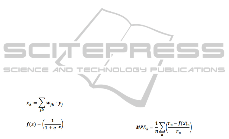
accomplished by an activation function and the

second one by a transfer function. The answer given

by the activation function is the result of adding the

various inputs which enter a certain neuron,

previously multiplied by their corresponding weights

(equation 1). The obtained result is then introduced

into the transfer function. The one selected was the

sigmoid function (equation 2), which offers

normalized results in the range (0, 1) (Knoerzer et

al., 2011).

(1)

(2)

In the equations above, w represents the weight,

y is the fed-forward signal, and x and f(x) symbolize

the activation function and transfer function

solutions respectively.

After these steps, the determination of the certain

statistical errors allows the optimization of the

weights to begin with the use of a training algorithm

or function (vide infra) (Demuth et al., 2005).

Once the optimization of the weights (training

phase) has concluded, the verification phase starts.

This phase, which does not involve any weight value

modification, gives an idea of how well the network

can generalize for data outside the training phase

dataset. Therefore, in order to develop this second

step of a training cycle or epoch, a new dataset is

employed, which is the verification dataset. The

trained ANN provides output signals which are

compared to the real values to obtain a verification

prediction error. Once this process ends, a training

cycle or epoch finishes, and a new one can start by

having the ANN process the training phase database

again. New training and verification cycles are done

in order to lower the verification prediction error as

much as possible, and only when this error starts to

grow, the training epochs stop, and the ANN can be

thought of as optimized (Demuth et al., 2005).

To sum up, in order to obtain a useful

mathematical model based on ANNs, a

representative database is required. It must be

divided into training and verification datasets

allowing the two steps of an epoch to take place

(training and verification phases).

Obtaining an ANN that is able to analyze a great

variety of nonlinear processes in the range of the

training dataset is desired. To avoid over-fitting

effects (custom-made networks that are only

accurate for data in the training dataset) and to

improve the generalization capability of the model,

small network topologies were selected, and the

trainBR training function was used. The trainBR

function improves the typical ANN generalization

because it updates the weights of the network by

analyzing the errors and the sum of the squares of

the network weights which allows finding the most

important parameters of the ANN and optimizes

them (Demuth et al., 2005; Torrecilla et al., 2008).

Once all of the necessary training and

verification cycles end, using the verification dataset

for simulation (not used for weight optimization),

the accuracy of the ANN is analyzed by calculating

the mean prediction error (MPE) (equation 3

(3)

In the equation above, MPE represents the mean

prediction error for a specific output neuron (k), n is

the number of data from the verification dataset, and

r and f(x) are the real and estimated output values

respectively.

2.3.1 Learning and Verification Datasets

Two databases have been used to optimize the ANN

models used:

The first database employed, which was to create

an ANN model to classify the desired VOCs (vide

supra), contains 1089 data points. The database was

split into two datasets which were the learning (925

data points) and the verification datasets (164 data

points). Every data point is characterized by seven

independent variables or inputs that are given by the

FET sensors used (various voltages and intensities),

and eleven dependent variables to classify the

specific compound. Every one of the eleven outputs

VolatileOrganicCompoundDetectionwithFETSensorsandNeuralNetworkDataProcessingasaPreliminaryStepto

EarlyLungCancerDiagnosis

has a specific value of 1 or 0. For instance, hexane

and octanol had a value of 1 for the second and the

eleventh variable respectively, and 0 for the

remaining ones. Therefore, hexane and octanol are

characterized by (0, 1, 0, 0, 0, 0, 0, 0, 0, 0, 0) and (0,

0, 0, 0, 0, 0, 0, 0, 0, 0, 1) vectors respectively.

For the ANN model used to estimate the partial

pressures of every compound, the database utilized

was formed by 1628 data points. Again, the database

was divided into two datasets which are the learning

(1364 data points) and verification datasets (264 data

points). The database contains information from

every FET sensor (HEX, HEP, DEC, and LAU),

compound (decane, hexane, mesitylene, octane,

butyl ether, chlorobenzene, cyclohexanone, decanol,

ethanol, hexanol, and octanol) and partial pressure

combination possible. Approximately ten

measurements were done for each available

combination. Every data point is formed by the

seven mentioned FET-related inputs and a single

output which is the partial pressure of the compound

in the analyzed sample.

Every ANN employed during the research was

designed using the software Matlab version

7.0.1.24704 (R14) (Demuth et al., 2005).

3 RESULTS

3.1 Field-Effect Transistor Sensor

Signals

The signals the different SiNW FET sensors

provided (measurable voltages and current

intensities) were the result of the interaction of the

VOCs and the molecular layers present in the

sensors. The produced interactions are noncovalent,

and can be classified into three distinct types:

dipole-dipole interactions between the molecular

layer and polar VOCs, induced dipole-dipole

interaction between the molecular layers and

nonpolar VOCs, and a tilt of the molecular layer

resulting from the diffusion of both kinds of VOCs

(Wang et al., 2013).

3.2 Artificial Neural Network Models

The design, optimization, and verification of the two

different MLP models created were done using the

data originated by the FET sensors (voltage and

current signals). The first model was done to classify

seven polar (butyl ether, chlorobenzene,

ciclohezanone, decanol, ethanol, hexanol, and

octanol) and four nonpolar (decane, hexane,

mesitylene, and octane) compounds, while the

second one was used to estimate the partial pressures

of the previously mentioned molecules, using the

data from the different FET sensors. The

calculations for this second model were done

depending on the kind of FET sensor (HEX, HEP,

DEC, and LAU) and the chemical nature of each

molecule studied. These two different models will

be explained separately in this section.

For both neural network models, the same two

stage calculation procedure was followed. The first

step consisted of statistically optimizing the main

parameters of the ANN using a thorough

experimental design. These parameters are the

hidden neuron number (HNN, number of neurons in

the hidden layer), the Marquardt adjustment

parameter (Lc), the decrease factor for Lc (Lcd), and

the increase factor for Lc (Lci) (Demuth et al.,

2005). The Lc parameter is similar to the learning

coefficient in the classic back-propagation

algorithms (Palancar et al., 1998). Its value is

respectively increased or decreased by Lci and Lcd

until these changes result in a reduced performance

value, which is measured with the MPE (equation

3) (Demuth et al., 2005). It is important to note that

finding the best results is not the goal, because the

real aim is to come across a solution which is good

enough to solve the defined problem (Oliferenko et

al., 2013). Once the values of these parameters have

been optimized, leading to a more accurate model,

the verification processes are applied to test the

networks using the verification datasets.

3.2.1 ANN1: Compound Classification

(Classifier)

The neural network used is a MLP which is formed

by three layers (vide supra) with seven input nodes,

some hidden neurons (HNN optimization shown

below), and eleven output neurons. The seven input

nodes of the MLP were used to insert the main

characteristics of every FET sensor tested as the

independent variables of the ANN model. These

inputs were different voltages and current intensities

that were measured after the VOCs interacted with

the FET sensors. On the other hand, the eleven

output neurons were used to classify every molecule

(vide supra). Using these output neurons, which

offer values of 0 or 1, a 1x11 vector is created. Each

vector corresponds to a specific compound.

The activation (equation 1), transfer (sigmoid

function, equation 2), and training (trainBR)

functions, which have been described before, are the

basis of the ANN used. The sigmoid function was

NCTA2014-InternationalConferenceonNeuralComputationTheoryandApplications

selected due to the ranges of the independent

variables selected. The trainBR function, also known

as the Bayesian regulation function, is the most

suitable function to avoid possible over-fitting

effects and to obtain an ANN with an acceptable

generalization capacity and a high applicability.

More specifically, the Bayesian regularization

function is a modified version of the Levenberg-

Marquardt training algorithm (trainLM) which

allows the network to generalize better. Using this

training function, the difficulty of defining the

optimum network architecture is reduced (Demuth et

al., 2005).

To compare the power and effectiveness of every

FET sensor, the same topology, parameters, and

initial weight values were tested in all devices tried

(HEX, HEP, DEC, and LAU). The optimal values of

the main parameters of the ANN have been

estimated through a meticulous experimental design

based on the Box-Wilson Central Composite Design

+ star points. The experimental parameters

analyzed were Lc, Lcd (both between 1 and 0.001),

Lci (between 2 and 100), and HNN. Taking the

learning dataset size into account, the HNN range

selected was between 2 and 10 neurons. The

optimized parameters are shown in table 2. Using

the verification dataset to simulate the model, no

misclassifications were found.

Table 2: Main parameters of both neural network models

used.

Parameters

Optimized values

ANN1 -

Classifier

ANN2 -

Estimator

Transfer function Sigmoid

Training function TrainBR

Hidden neuron

number

4 5

Lc 0.01 0.001

Lcd 0.1 0.02

Lci 10 5

3.2.2 ANN2: Estimation of the Partial

Pressure of Polar and Nonpolar VOCs

(Estimator)

In this section, ANN models to estimate the partial

pressure of nonpolar (decane, hexane, mesitylene,

and octane) and polar (butyl ether, chlorobenzene,

ciclohezanone, decanol, ethanol, hexanol, and

octanol) compounds are presented. The models used

are MLPs, similar to the ones described in the

previous section. The three-layer ANN models

tested have seven input nodes and one output

neuron. The same mentioned seven FET-related

independent variables are inputted into the neural

network model and the estimation of the partial

pressure of every molecule is provided by a single

output neuron.

The combination of every FET sensor type

(HEX, HEP, DEC, and LAU) with each compound

estimated (decane, hexane, mesitylene, octane, butyl

ether, chlorobenzene, ciclohezanone, decanol,

ethanol, hexanol, and octanol) originated 44

networks. To test the power and usefulness of every

FET sensor employed, only one set of values of the

main neural network parameters (topology, Lc, Lcd,

and Lci) has been selected and used for all 44

networks resulting from all possible sensor-

compound combinations. The parameter

optimization was achieved with an experimental

design based on the Box-Wilson Central Composite

Design 2

+ star points. The experimental factors

analyzed were Lc, Lcd (both between 1 and 0.001),

Lci (between 2 and 100), and HNN. Due to the

learning dataset size, the HNN range selected was

again between 2 and 10. All the parameters were

chosen in order to achieve the least value of MPE

possible (equation 3). The optimized parameter

values are shown in table 2. In addition, after using

the optimized neural network parameters, the

weights of each connection were optimized and

validated to estimate the partial pressure of every

compound with the least prediction error. The MPE

values calculated during the 44 verification

processes are shown in table 3.

4 DISCUSSION

4.1 ANN1: Compound Classification

(Classifier)

Analyzing the results of the ANN used to classify

the different molecules, no mistakes or

misclassifications have been found. Therefore, the

optimized MLP model is able to discriminate

perfectly all eleven of the tested compounds. It is

important to additionally acknowledge that these

statistical results imply that the neural network

tested is not only a suitable tool to classify the

compounds studied as polar or nonpolar, but also it

is capable of distinguishing among every specific

molecule used in terms of its chemical nature. This

means that for all eleven types of VOCs studied,

individual and clearly distinguishable vectors were

provided by the MLPs.

VolatileOrganicCompoundDetectionwithFETSensorsandNeuralNetworkDataProcessingasaPreliminaryStepto

EarlyLungCancerDiagnosis

4.2 ANN2: Estimation of the Partial

Pressure of Polar and Nonpolar

VOCs (Estimator)

The MPE values shown in table 3 lead us to state

that the simple ANN models tested are more than

adequate tools to estimate the partial pressures of

polar and nonpolar compounds by most of the FET

sensors tested. The LAU FET sensor offers the best

performance in terms of estimating the partial

pressure of the nonpolar compounds. This sensor

offered the lowest MPE values for the estimation of

two determined nonpolar compounds (decane and

hexane) and two polar compounds (ethanol and

hexanol). Alternatively, The HEP FET sensor is the

best one when estimating the partial pressure of

polar compounds (best performance in three out of

seven polar compounds).

In general terms, it can be observed that the

estimation of the partial pressures of polar VOCs

offer better results than the nonpolar ones. To try to

explain this fact, the stronger interactions the polar

compounds present with the functionalized SiNW

FET sensors when compared to the interactions of

the nonpolar compounds may lead to more specific

signals. As mentioned before, the polar VOCs

interact through dipole-dipole interactions, while the

nonpolar VOCs interact with induced dipole-dipole

ones (Wang et al., 2013), which are far weaker and,

therefore, probably offer less repetitive signals.

To sum up, specific combinations of FET sensors

and ANNs are able to estimate the partial pressure of

every polar and nonpolar VOC analyzed with MPEs

between 3.3 and ~0% (Table 3). The used MLP

models thus result in reliable and accurate

chemometric tools for processing the databases

produced by the FET sensors.

Table 3: MPE values of the verification of every FET-ANN combination optimized (the best sensor in each compound is

shown in bold).

Nonpolar Polar

Chemical FET Sensor MPE (%) Chemical FET Sensor MPE (%)

Decane

HEX 2.1

Butyl ether

HEX 2.4

HEP 3.6

HEP

0.02

DEC 1.5 DEC 1.4

LAU

1.2 LAU 6.3

Hexane

HEX 3.9

Chlorobenzene

HEX

1.3

HEP 5.1 HEP 6.5

DEC 4.8 DEC 2.1

LAU

3.3 LAU 13.6

Mesitylene

HEX 10.7

Cyclohexanone

HEX 0.9

HEP 4.1

HEP

≈0

DEC

2.8 DEC 1.8

LAU 43 LAU 1.8

Octane

HEX

0.2

Decanol

HEX

0.3

HEP 6.1 HEP 2.3

DEC 1.4 DEC 0.8

LAU 20.7 LAU 2.6

Ethanol

HEX 2.3

HEP 4.0

DEC 2.5

LAU

1.9

Hexanol

HEX 0.1

HEP 0.08

DEC 1.6

LAU

≈0

Octanol

HEX 1.9

HEP

1.1

DEC 2.5

LAU 2.6

NCTA2014-InternationalConferenceonNeuralComputationTheoryandApplications

5 CONCLUSIONS

A preliminary step for early, fast, sensitive, and

noninvasive LC diagnosis based on biomarkers in

breath has been looked into and described. It has

been proven that the combination of functionalized

SiNW FET sensors and ANNs are able to more than

adequately classify the eleven different polar and

nonpolar VOCs studied and accurately estimate their

partial pressures in artificial gaseous samples. The

neural network models of the databases generated by

the FET sensors provided a perfect classification of

the analyzed VOCs (ANN1) and the possibility to

determine their partial pressures with MPEs never

greater than 3.3% (ANN2), which consequently

validates both the classifier (ANN1) and the

estimator (ANN2) models.

These promising results open a door to further

research with artificial breath and, in the end, real

breath samples. The final goal of this project is to

precisely define the biomarker profiles in breath of

healthy controls and LC patients and, ideally, the

profiles of every LC stage to be able to detect

potential LC patients and diagnose this disease at the

earliest stage possible. This assisted diagnosis could

help the medical staff make decisions and

conceivably allow identifying early and, most

importantly, curable LC cases.

ACKNOWLEDGEMENTS

The research leading to these results has achieved

funding from the European Union Seventh

Framework Programme (FP7/2007–2013) under

grant agreement no. HEALTH-F4-2011-258868.

REFERENCES

Anand, P., Kunnumakara, A. B., Sundaram, C.,

Harikumar, K.B., Tharakan, S. T., Lai, O. S., Sung, B.,

Aggarwa, B. B. (2008) ‘Cancer is a Preventable

Disease that Requires Major Lifestyle Changes’,

Pharm. Res., vol. 25, no. 92, pp.097-2116.

Blase, X., Serra-Fernández, M. V. (2008) ‘Preserved

Conductance in Covalently Functionalized Silicon

Nanowires’, Physical Review Letters, vol. 100, no. 4.

Cancilla, J. C., Torrecilla, J. S., Matute, G. (2014)

‘Current Applications of Artificial Neural Networks in

Biochemistry with Emphasis on Cancer Research’,

Curr. Biochem. Eng., vol. 1.

Chen, K. I., Li, B. R., Chen, Y. T. (2011) ‘Silicon

Nanowire Field-Effect Transistor-Based Biosensors

for Biomedical Diagnosis and Cellular Recording

Investigation’, Nano Today, vol. 6, pp. 131-154.

Cui, Y., Zhong, Z., Wang, D., Wang, W.U., Lieber, C.M.

(2003) ‘High Performance Silicon Nanowire Field

Effect Transistors’, Nano Letters, vol. 3, no. 2.

Demuth, H., Beale, M., Hagan, M. (2005) ‘Neural

Network Toolbox for Use with MATLAB® User’s

Guide’. Version 4.0.6. Ninth printing Revised for

Version 4.0.6 (Release 14SP3), Natick, MA (USA).

Desai, K. M., Survase, S. A., Saudagar, P. S., Lele, S. S.,

Singhal, P.S. (2008) ‘Comparison of Artificial Neural

Network (ANN) and Response Surface Methodology

(RSM) in Fermentation Media Optimization: Case

Study of Fermentative Production of Scleroglucan’,

Biochem. Eng. J., vol. 41, num. 3, pp. 266-273.

Farrington, S. M., Lin-Goerke, J., Ling, J., Wang, Y.,

Burczak, J. D., Robbins, D. J., Dunlop, M. G. (1998)

‘Systematic Analysis of hMSH2 and hMLH1 in

Young Colon Cancer Patients and Controls’, Am. J.

Hum. Genet., vol. 63, pp. 749-759.

Flores-Fernández, J. M., Herrera-López, E. J., Sánchez-

Llamas, F., Rojas-Calvillo, A., Cabrera-Galeana, P.A.,

Leal-Pacheco, G., González-Palomar, M. G., Femat,

R., Martínez-Velázquez, M. (2012) ‘Development of

an Optimized Multi-biomarker Panel for the Detection

of Lung Cancer Based on Principal Component

Analysis and Artificial Neural Network Modeling’,

Expert Syst. Appl., vol. 39, no. 12, pp. 10851-10856.

Gueguim-Kana, E. B., Oloke, J. K., Lateef, A., Adesiyan,

M.O. (2012) ‘Modeling and optimization of biogas

production on saw dust and other co-substrates using

Artificial Neural network and Genetic Algorithm’,

Renew. Energy., vol. 46, pp. 276-281.

Jain, A. K., Mao, J., Mohiuddin, K. M. (1996) ‘Artificial

Neural Networks: A Tutorial’, Computer, vol. 29, no.

3, pp. 31-44.

Jemal, A., Bray, F., Center, M. M., Ferlay, J., Ward, E.,

Forman, D. (2011) ‘Global Cancer Statistics’, CA

Cancer J. Clin., vol. 61, pp. 69-90.

Knoerzer, K., Juliano, P., Roupas, P., Versteeg, C. (2011)

‘Innovative Food Processing Technologies: Advances

in Multiphysics Simulation’, Oxford (UK), Wiley-

Blackwell.

Li, Y., Qian, F., Xiang, J., Lieber, C. M. (2006) ‘Nanowire

Electronic and Optoelectronic Devices’, Materials

Today, vol. 9, no. 10.

McGrath, M., Lee, I. M., Buring, J., De-Vivo, I. (2011)

‘Common Genetic Variation Within IGFI, IGFII,

IGFBP-1, and IGFBP-3 and Endometrial Cancer Risk’

Gynecol. Oncol., vol. 120 no. 2, pp. 174-178.

Oliferenko, A. A., Oliferenko, P. V., Torrecilla, J. S.,

Katritzkya, A. R. (2013) ‘Rebuttal to “comments on

“Boiling Points of Ternary Azeotropic Mixtures

Modeled with the Use of Universal Solvation Equation

and Neural Networks”’, Industrial & Engineering

Chemistry Research, vol. 52, pp. 545-546.

Palancar, M. C., Aragon, J. M., Torrecilla, J. S. (1998)

‘pH-Control System Based on Artificial Neural

Networks; Industrial & Engineering Chemistry

Research’, vol. 37, no. 7, pp. 2729-2740.

VolatileOrganicCompoundDetectionwithFETSensorsandNeuralNetworkDataProcessingasaPreliminaryStepto

EarlyLungCancerDiagnosis

Parmigiani, G., Berry, D. A., Aguilar, O. (1998)

‘Determining Carrier Probabilities for Breast Cancer-

Susceptibility Genes BRCA1 and BRCA2’, Am. J. of

Hum. Genet., vol. 62, no. 1, pp. 145-158.

Paska, Y., Haick, H. (2009) ‘Controlling properties of

field effect transistors by intermolecular cross-linking

of molecular dipoles’, Applied Physics Letters, vol.

95.

Peled, N., Hakim, M., Bunn, P. A., Miller, Y. E.,

Kennedy, T.C., Mattei, J., Mitchell, J. D., Hirsch, F.

R., Haick, H. (2012) ‘Non-invasive Breath Analysis of

Pulmonary Nodules’, J. Thorac. Oncol., vol. 7, pp.

1528-1533.

Peng, G., Trock, E., Haick, H. (2008) ‘Detecting

Simulated Patterns of Lung Cancer Biomarkers by

Random Network of Single-Walled Carbon Nanotubes

Coated with Nonpolymeric Organic Materials’, Nano

Letters, vol. 8, no. 11, pp. 3631-3635.

Peng, G., Tisch, U., Adams, O., Hakim, M., Shehada, N.,

Broza, Y. Y., Billan, S., Abdah-Bortnyak, R., Kuten,

A., Haick, H. (2009) ‘Diagnosing lung cancer in

exhaled breath using gold nanoparticles’, Nature

Nanotechnology.

Plass, K. E., Liu, X., Brunschwig, B. S., Lewis, N. S.

(2008) ‘Passivation and Secondary Functionalization

of Allyl-Terminated Si(111) Surfaces’, Chem. Mater.,

vol. 20, pp. 2228-2233.

Sze, S. M. (2001) ‘Semiconductor Devices; Physics and

Technology’, New York (USA), 2, John Wiley & Sons

Inc.

Tisch, U., Billan, S., Ilouze, M., Phillips, M., Peled, N.,

Haick, H. (2012) ‘Volatile Organic Compounds in

Exhaled Breath as Biomarkers for the Early Detection

and Screening of Lung Cancer’, CML – Lung Cancer,

vol. 5, no. 4, pp. 107-117.

Torrecilla, J. S., Aragón, J. M., Palancar, M. C. (2008)

‘Optimization of an Artificial Neural Network by

Selecting the Training Function. Application to Solid

Drying’, Industrial & Engineering Chemistry

Research, vol. 47, pp. 7072-7080.

Torrecilla, J. S., Sanz, P. D. (2011) ‘Neural Networks:

Their Role in High-Pressure Processing. Book Title:

Innovative Food Processing Technologies: Advances

in Multiphysics Simulation’ (Eds. Kai Knoerzer, Pablo

Juliano, Peter Roupas, Cornelis Versteeg) John Wiley

& Sons, Ltd. and Institute of Food Technologists.

Torrecilla, J. S., Tortuero, C., Cancilla, J. C., Díaz-

Rodríguez, P. (2013) ‘Estimation with Neural

Networks of the Water Content in Imidazolium-Based

Ionic Liquids Using their Experimental Density and

Viscosity Values’, Talanta, vol. 113, pp. 93-98.

Wang, B., Haick, H. (2013) ‘Effect of Functional Groups

on the Sensing Properties of Silicon Nanowires toward

Volatile Compounds’, ACS Appl. Mater. Interfaces,

vol. 5, pp. 2289-2299.

Wu, Yo., Wu, Yi., Wang, J., Yan, Z., Qu, L., Xiang, B.,

Zhang, Y. (2011) ‘An Optimal Tumor Marker Group-

Coupled Artificial Neural Network for Diagnosis of

Lung Cancer’, Expert Syst. Appl., vol. 38, no. 9, pp.

11329-11334.

NCTA2014-InternationalConferenceonNeuralComputationTheoryandApplications